Deep Learning for Computer Vision Lecture 2
2022 Deep Learning for Computer Vision Lecture2
In this lecture, we will glance at Neural Networks & CNN. Let’s get started.
Recap: Linear Regression
Firstly we can recap the linear regression part. Let’s take the input image as $x$, and the linear classifier as $W$. We need$ y = Wx + b$ as a 10-dimensional output vector, indicating the score for each class.
Our computational Graph looks like this:
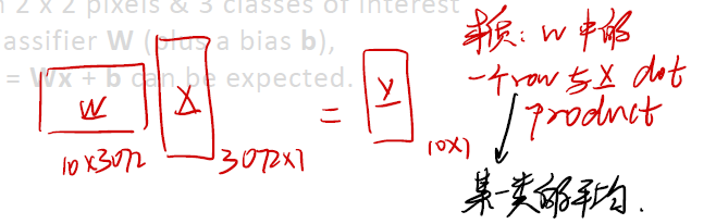
We have mentioned before, final result of $y$ is a dot product of a row in $W$ and a column in $x$. This is a kind of “average”. The $W$ has 10 rows, project to 10 types of final result. In this case, we can see the row as the average of a class.
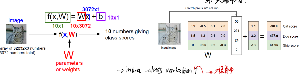
However, when using linear regression on image classification, we find problems. When the # of class increase, comes:
- intra-class variation $\uparrow$
- inter-class variation $\downarrow$
So how to deal with this problem?
Biological neuron and Perceptrons
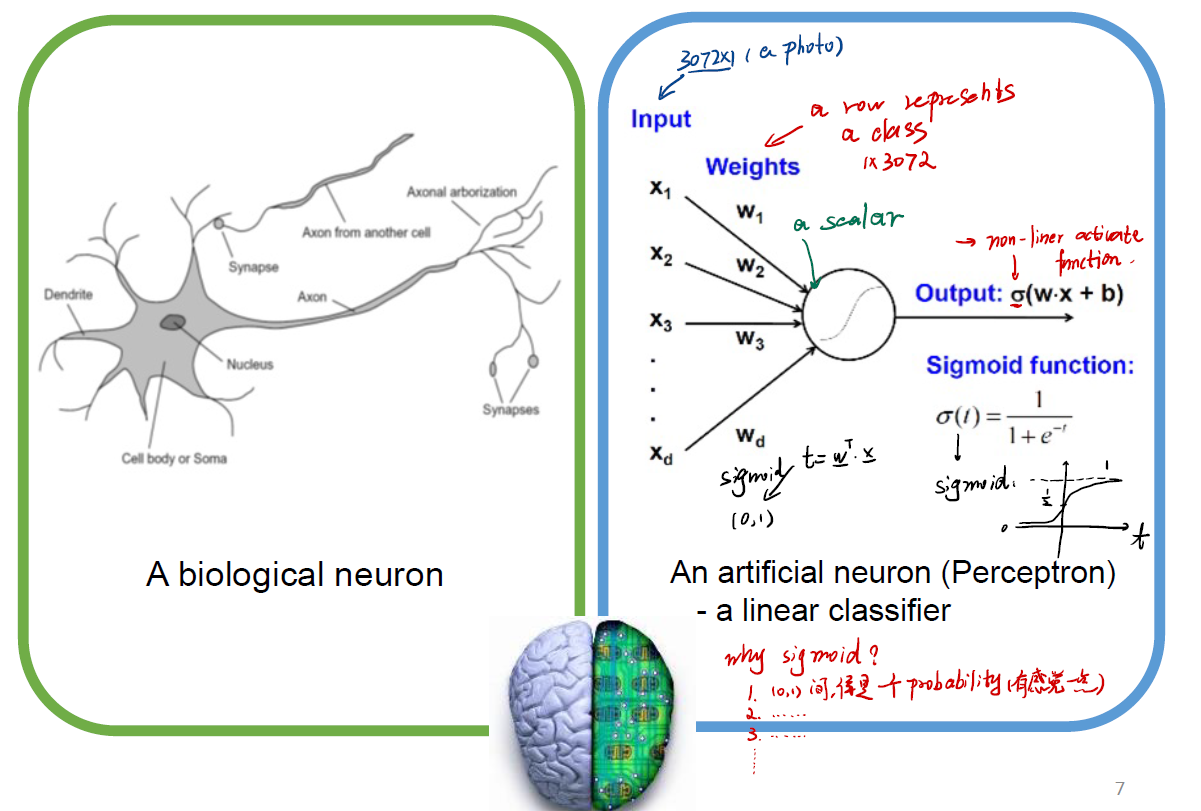
According to the concept of biological neuron, we may think that we can feed the input to a “neuron” in our computer. This neuron is, maybe, a function. We call it activate function.
And, choose what function as our activate function? we just use sigmiod function as it. This is a non-linear activate function. The form of sigmoid function is:
Mind that when $t \rightarrow \infty$, $\sigma(t) \rightarrow 1$, when $t \rightarrow -\infty$, $\sigma(t) \rightarrow 0$. It looks like a kind of probability!
Our model now can be written as:
\[y = \sigma(W^Tx + b)\]and we just need to learn $W$.
Not fast, but deep
We also want to learn again and again. This means that we need lots of layers! Multi-Layer Perception/Neural Network comes…
We use input $x$, and $x$ goes through hidden layer $1, 2, … n$, till final output layer $y$.
This is so called deep.
Hierarchical Representation Learning
Successive model layers learn deeper intermediate representations.
For example, we want to learn faces. Use 3 layers:
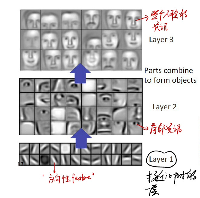
- Layer 1 is the nearest to our input. We can visualize it below. It seems that the layer 1 have already learnt some “direction feature”. Maybe, the eyes direction.
- Layer 2 use layer 1 as its input. Now we can find that it learnt some
local information! Eyes, noses, and so on. - Layer 3 has the hole faces information.
It is clearly that, when our model goes to deep, every layer can learn some feature. And to be more concise, the feature becomes more and more complex. From direction to faces.
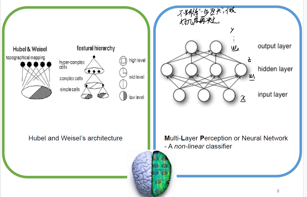
Multi-layer Perceptron: A Nonlinear Classifier
Now let’s see an example of Multi-layer Perceptron.
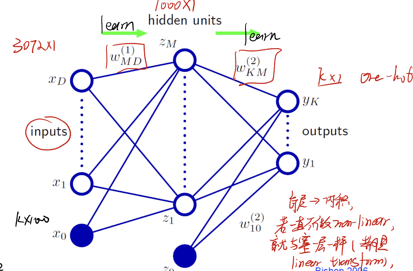
We have input left and output right, with hidden units. When learning, we need to learn two sets of parameters:
- $w_{MD}^{(1)} … w_{10}^{(1)}$: inputs $x_1, … ,x_D$ to hidden layer.
- $w_{KM}^{(2)}, …, w_{10}^(2)$: hidden layer to outputs.
So there comes a question: where shall we put our activation function on?
Of course we need to put the activation functions in each layer! Mind that in every layer, we actually do $W^{(1)^T}x + b$. If we were not going to add activation function on each layer, we may have:
\[W^{(2)^T}(W^{(1)^T}x + b_1) + b_2\]actually, this can not use the advantage that we design two layers. Just one layer can also fulfill this form! Otherwise, with activation function added to each layer, we get:
\[\text{output} = \sigma(W^{(2)^T}\sigma((W^{(1)^T}x + b_1)) + b_2)\]This is useful when learning.
Take a closer look…
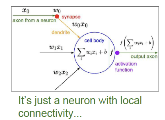
Let’s take a neuron for an example.
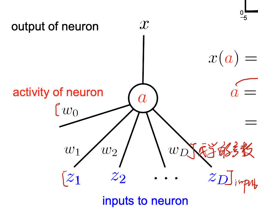
For this neuron, we have:
- input: $z_1, z_2, …, z_D$. A $D$-dimension vector.
- output: a real number $x$.
- parameters to be learnt: $w_0, w_1, …, w_D$
Input-Output Function of a Single Neuron
For a single neuron, let’s take a look.
Assume that:
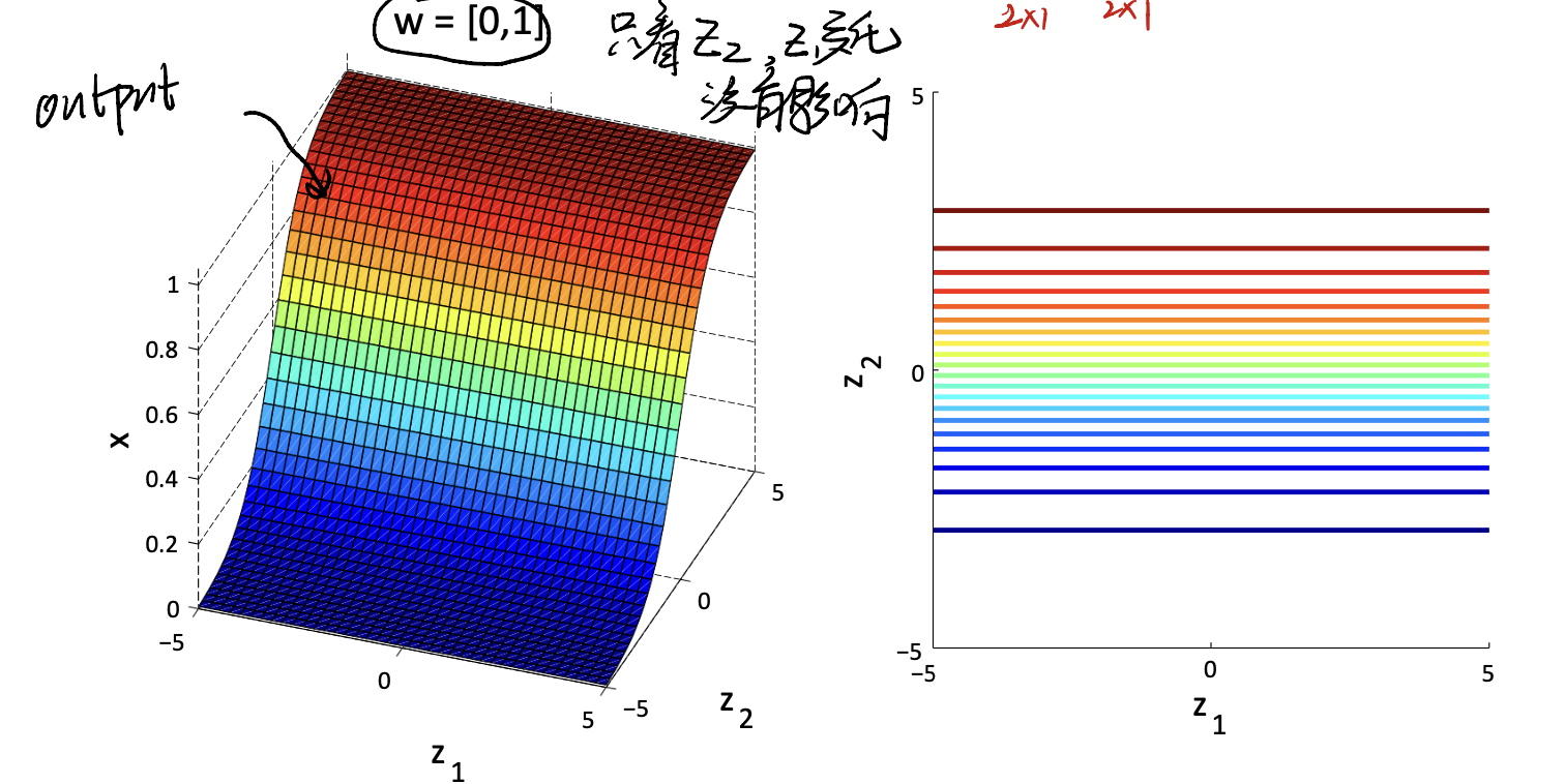
\[x(z_1,z_2) = \frac {1} {1 + \exp(-w_1z_1 - w_2z_2)}\]and set parameter $w = (0, 1)$
we can see that in this case, only input $z_2$ works. And our output value like:
If we change $w = (0.2, 1)$, we have:

| It rotates. and so on, so forth. And if we add constrains like $ | w | \leq k$, we can set other boundaries: |
$w / w $ sets direction of boundary. $ w $ sets steepness of boundary.
Training a Single Neuron
After all, our target is training and predicting. So it’s time to see how to train a single neuron.
Firstly, we shall need to define the input and output.
- input: $\mathbf{z} = (z_1, z_2)$
- output: $\mathbf{x} = 1,0$
Next, our model is a linear model, so we can set model parameters:
- $w = (w_1, w_2)$
Third part is the objective function. In machine learning or deep learning, we always have our loss function. In this classification function, we can choose BCE loss, aka, Binary Cross Entropy.
Our objective function is:
\[G(\mathbf{w}) = -\sum_n [t^{(n)}\log x(z^{(n)}; w) + (1 - t^n)\log (1 - x(z^{(n)}; w))]\]where $t^{(n)}$ is our classification indicator.
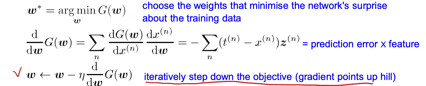
How do we learn the model $w$? use gradient decent to help.
Overfitting and Weight Decay
We, always face overfitting problem. If we want to cut overfitting, we shall add some “regulization”.
Let’s change our optimization constrains:
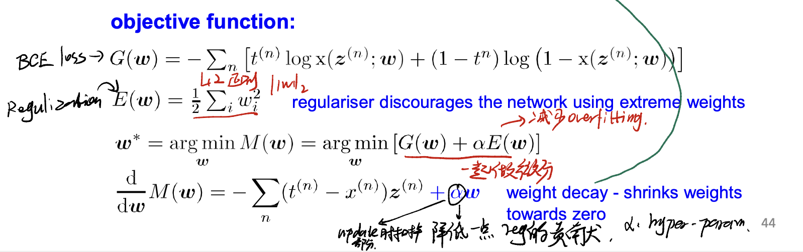
This method is called weight decay method. It will shrinks weights towards zero, so the model will not be too complicated, and we can avoid several overfitting problem.
L1-norm and L2-norm
There are two constrains we often use. L1-norm and L2-norm.
L1-norm constrain is:
\[||w||_1 \rightarrow \sum |w_i|\]and L2-norm constrain is:
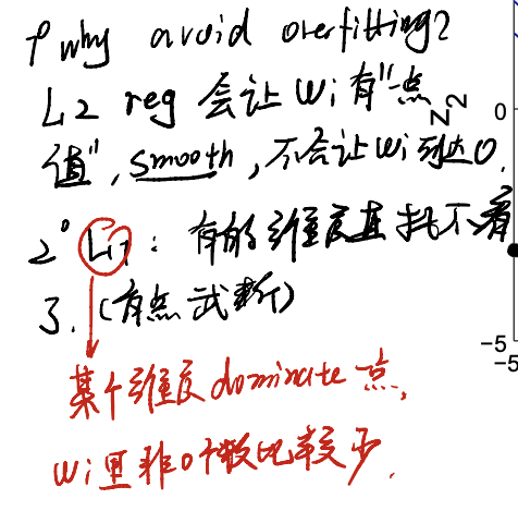
\[||w||_2 \rightarrow \sum w_i^2\]In particular, L1 norm will make sparse situation. Means that it will force some $w_i$ directly to zero. However, L2 norm will make average situation. Means that it will let $w_i$ be similar and smaller.
Training a Neural Network with a Single Hidden Layer
Networks with hidden layers can be fit using gradient descent using an algorithm called back-propagation.
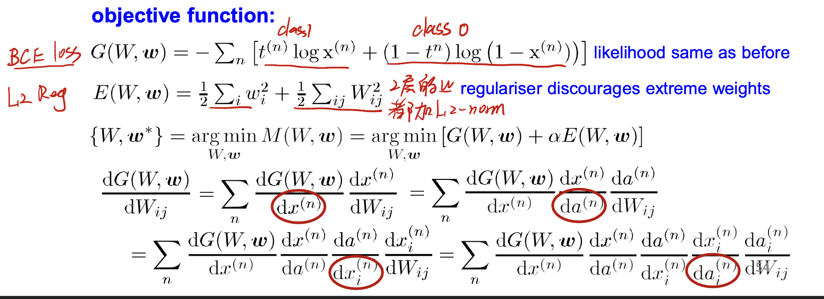
Mind that if we want to use regulization methods, we need to add each layer the constrain.(L2-norm)
Convolutional Neural Networks
Now, we can talk about CNN-Convolutional Neural Networks.
If, Multi-Layer Perceptron on images?
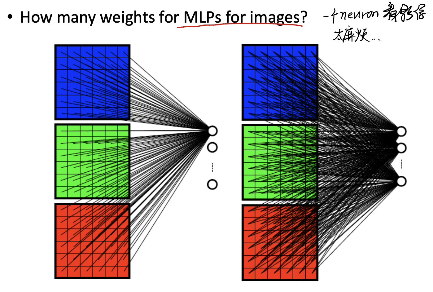
Too many weights we need to use for a neuron.
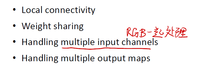
To handle this, CNN use two methods:
- Local Connectivity: Each neuron takes info only from a neighbourhood of pixels.
- Weight Sharing: Neurons connecting all neighbourhoods have identical weights.
let’s see them.
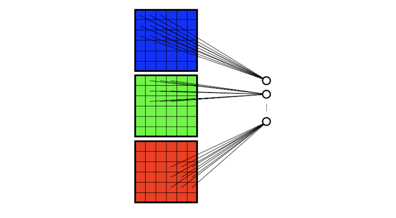
CNN: Local Connectivity
In our former model, we have “FC” Network, meaning “Fully Connected Network”. You can see this:
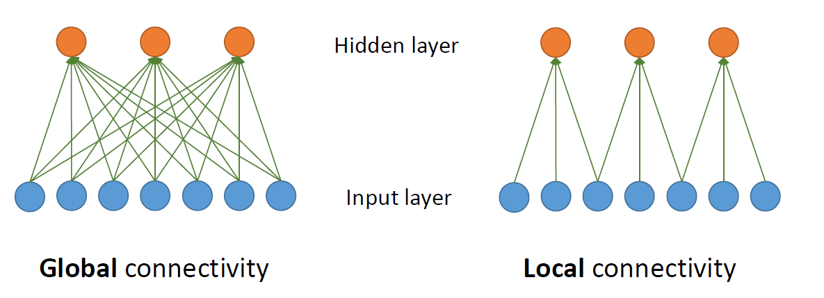
Assume that we have 7 input and 3 hidden units. See the # of parameters:
- Global connectivity: we will need to learn $3 \times 7 = 21$ parameters with a fully connected network.
- Local connectivity: in this case, we just let the first neuron see the first 3 inputs, the second neuron see the second 3 inputs, and the third neuron see the final three inputs.
With local connectivity, we can reduce the number of parameters!
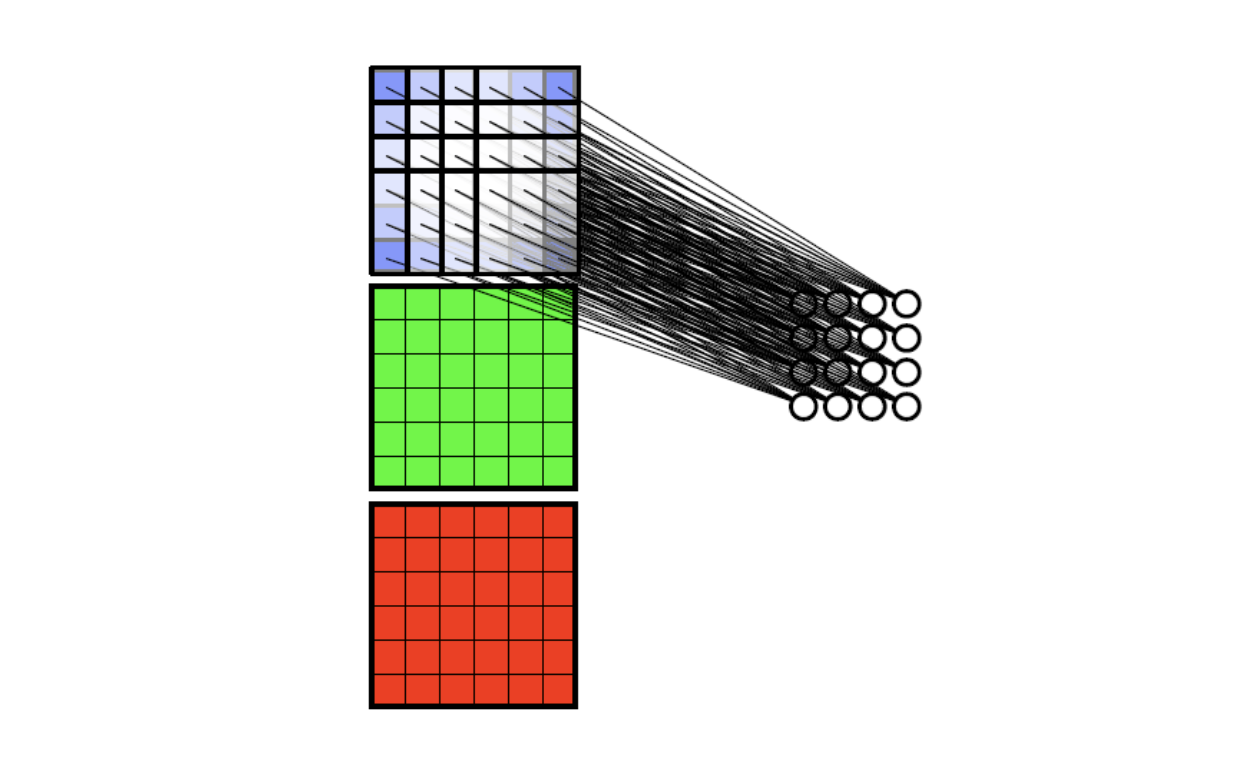
CNN: Weight Sharing
Weight Sharing is another useful technique. It can help us reduce the # of parameters again!
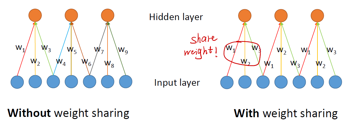
The idea of this technique is that a kernel’s duty is to detect a specific feature of an image. And, wherever the feature is, the same kernel can still successfully detect it. So, with the same weights, the kernel can detect the same pattern of an image.
In the picture, the orange nodes can be recognised as the output of a kernel.
CNN with Multiple Input Channels
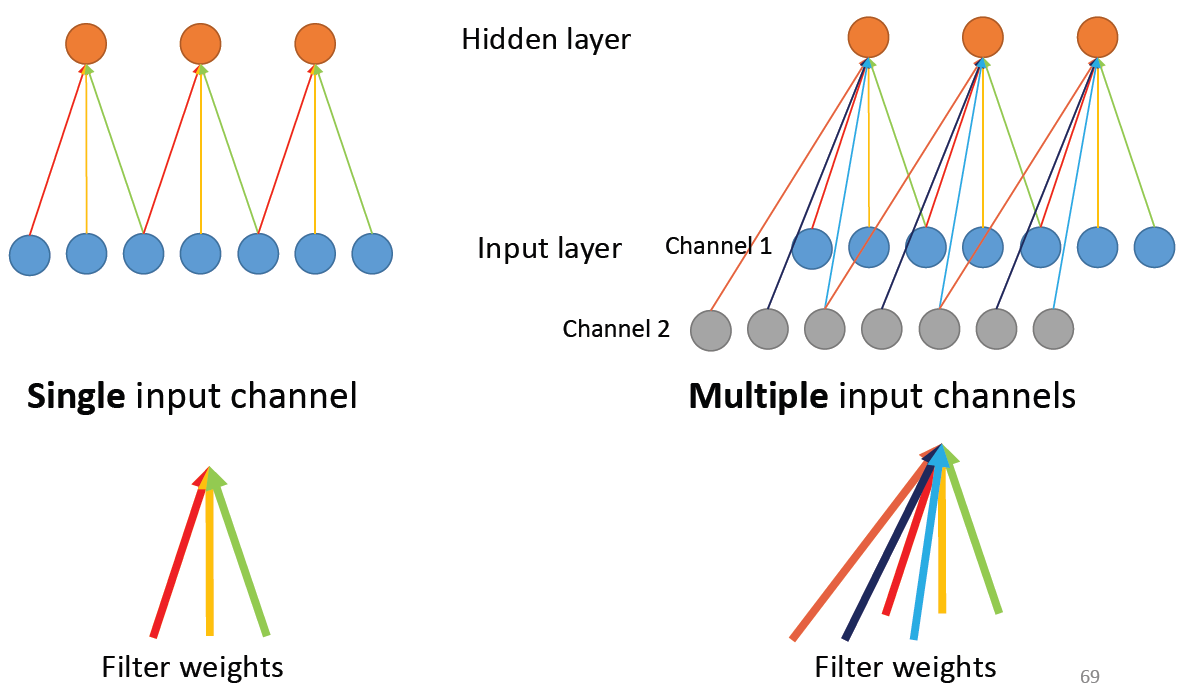
We can think of a single input channel as we are dealing with a grayscale image, with only one colour channel.
But in reality, the image has always three channels: R, G, and B. Each kernel’s output will need multiple channel’s data to join the calculation.
In the multiple channel case, the kernel will apply to each channel respectively, and add these calculation result, to form a feature map.
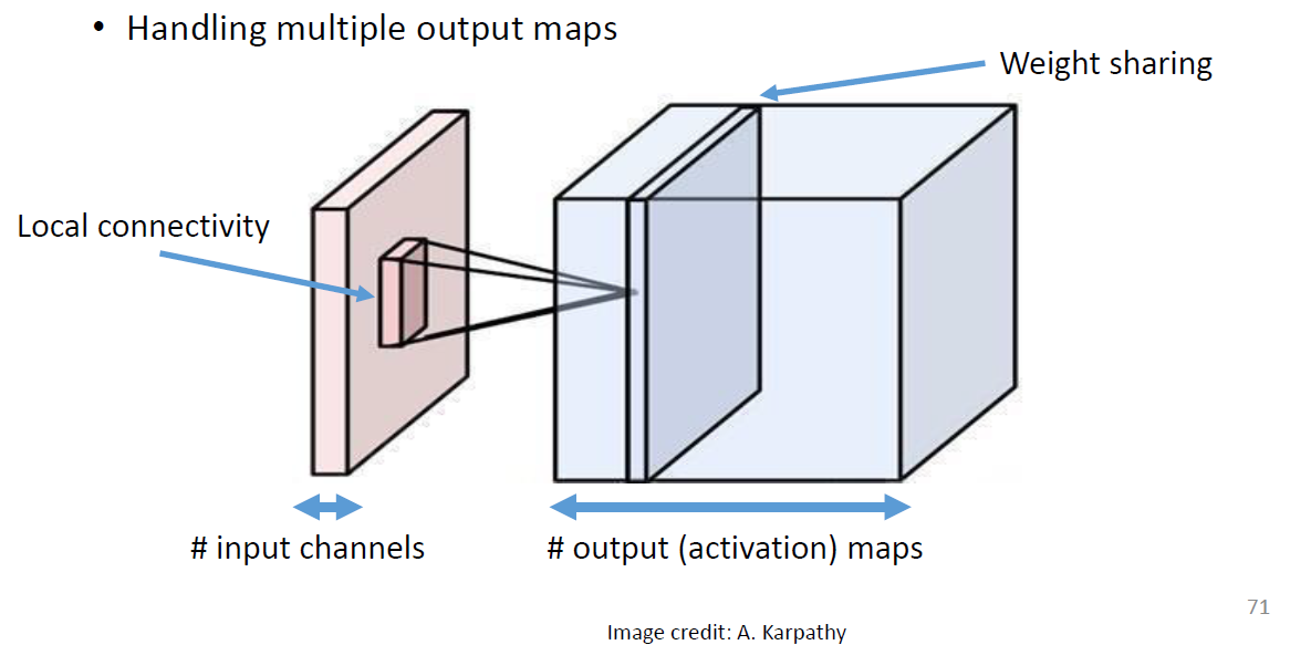
CNN with Multiple Output Maps
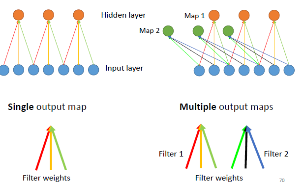
Actually, it means that each time we apply our convolutional kernel to an image, we can get a feature map output as our result. Multiple Output Maps technique allows the CNN to form multiple feature maps, capturing multiple different features.
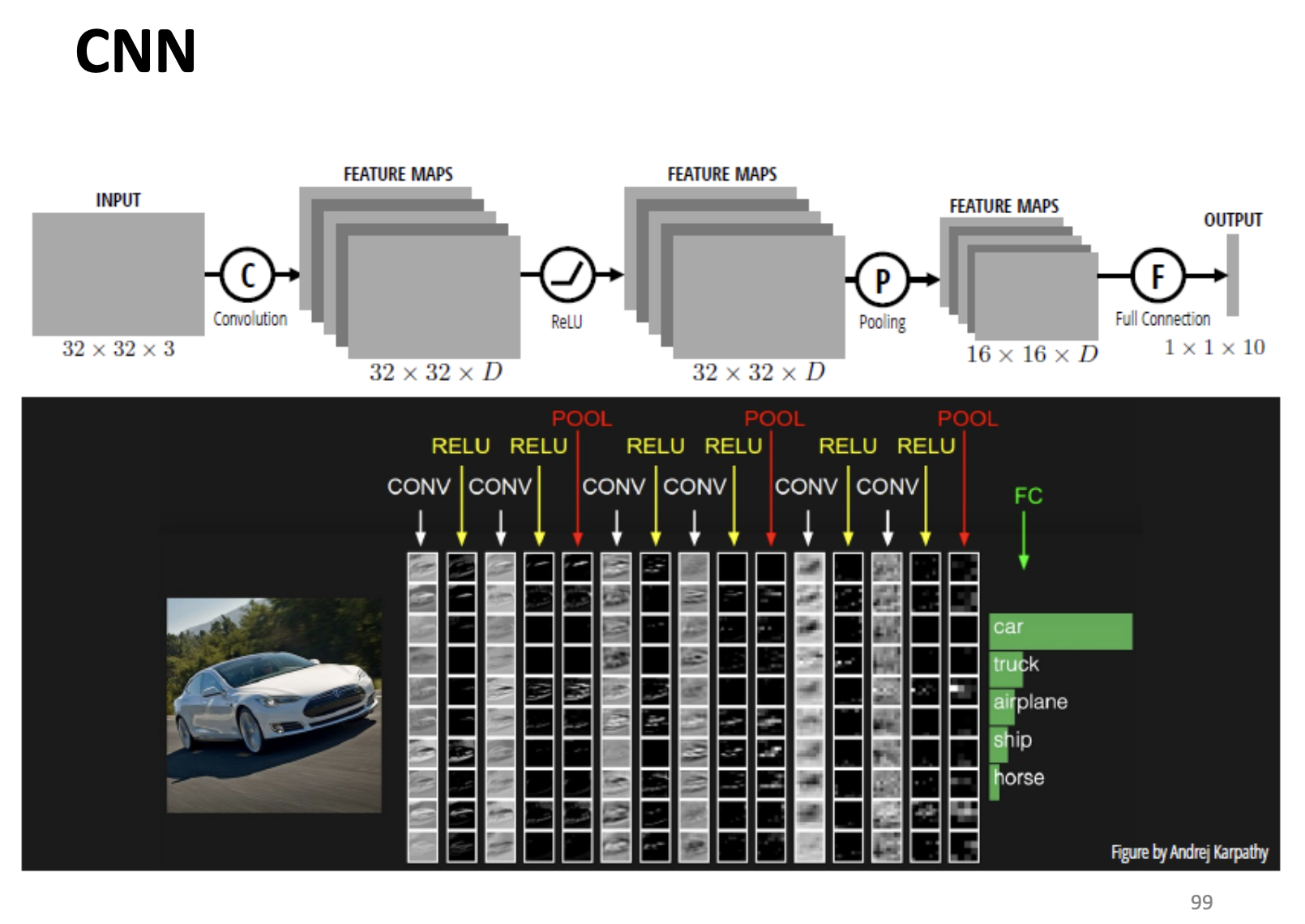
Putting them together::CNN
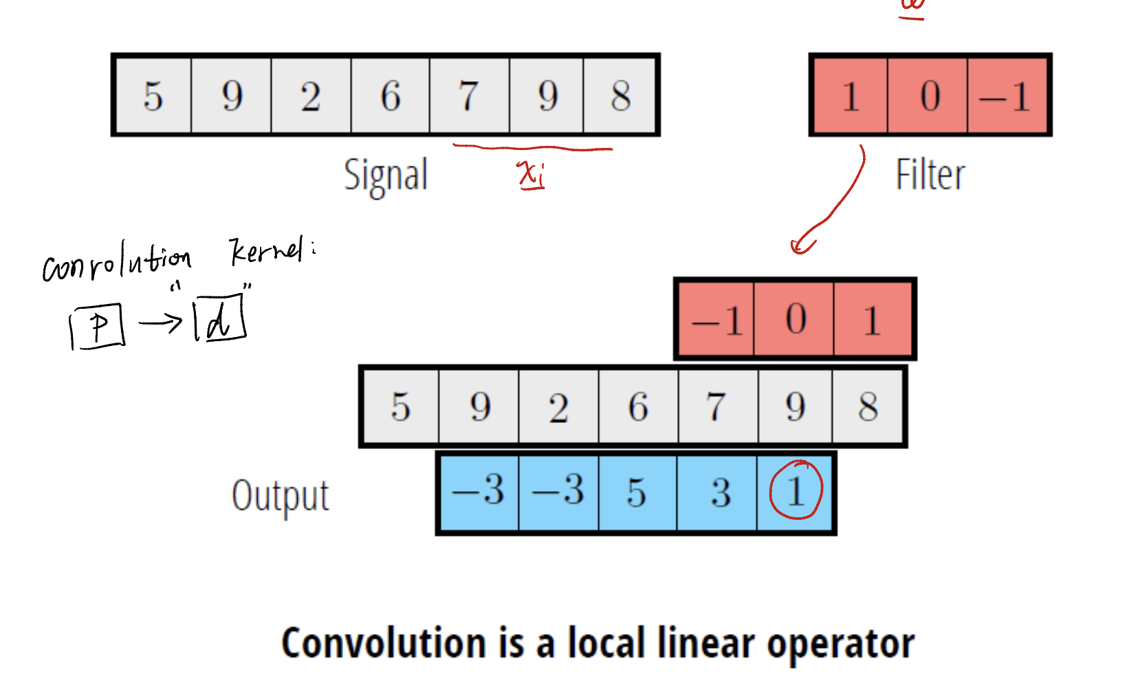
What is a Convolution?
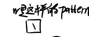
To know what is a convolution, we need to define what is a kernel in CNN.
Kernel
You can image a kernel as a little “feature graph”. For example, a $3 \times 3$ kernel may look like a square, with a feature:
In our learning process, we do the matrix multiply, just like:
\[\text{A pixel in the feature map} = W^T x_i\]This is the process when calculating a pixel in the next feature map. We just use the kernel $W^T$, and scan the whole origin image, to get a pixel of the next feature map.
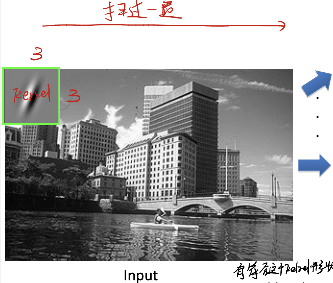
So we generate a feature map! It looks like:
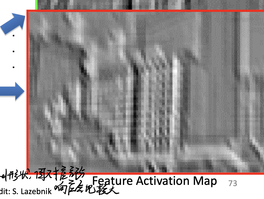
The idea is that if there’s a similar part(similar feature) in the original image, when the kernel scans through the part, it will generate a large response. This is shown in the feature map.
Kernel in Neuron View
Say that we have a $32 \times 32 \times 3$ image, and a $5 \times 5 \times 3$ filter(or kernel). We can generate a feature map by going through the whole image.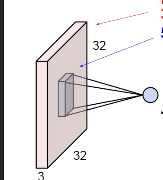
Hint: the channel of the kernel must match the input image’s channel.
It seems like a neuron! With few connections compared to the fully connected network.
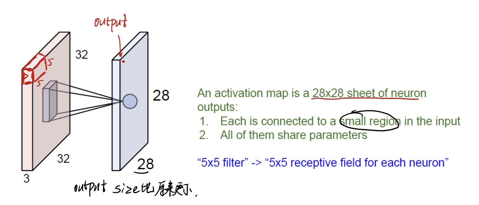
Must bear in mind that the output of the feature map is just a 2D-image. Not 3 channel image. And the size of the feature map is smaller than before.
Every layer maps every kernel
In part before, we mind that one kernel generates a “slides”. How about multiple kernels? What will they generate? Let’s see.
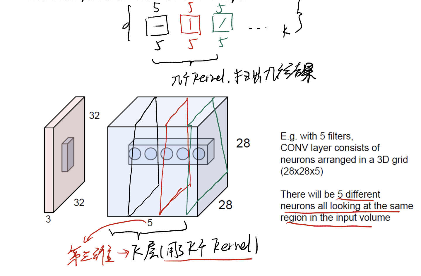
Image that we have already set $k$ kernel, each kernel is $5 \times 5 \times 3$ size. When we get all the slices of the feature map, we kan put them to getter! To generate a whole feature cube…
The feature cube now has $28 \times 28 \times k$, where k is the # of kernels.
Shrink!
Image input with $32 \times 32$ pixels convolved repeatedly with $5 \times 5 \times 3$ filters shrink volumes spatially. This is a kind of “dimension reduction”.
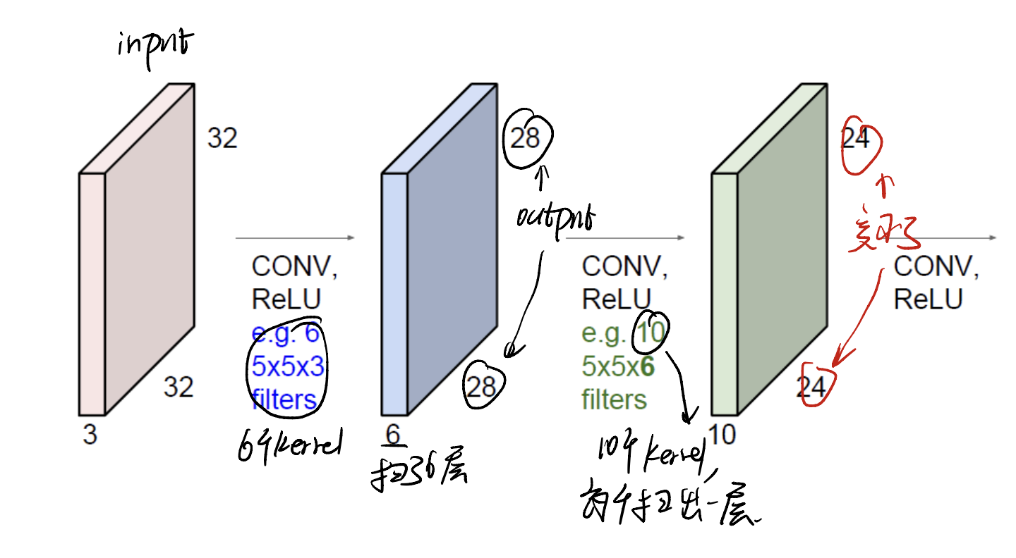
Why ReLU? Just because we want some non-linear feature.
Trick 1: Zero Padding
If we do not want the image to shrink, what can we do? Let’s see the zero padding trick.
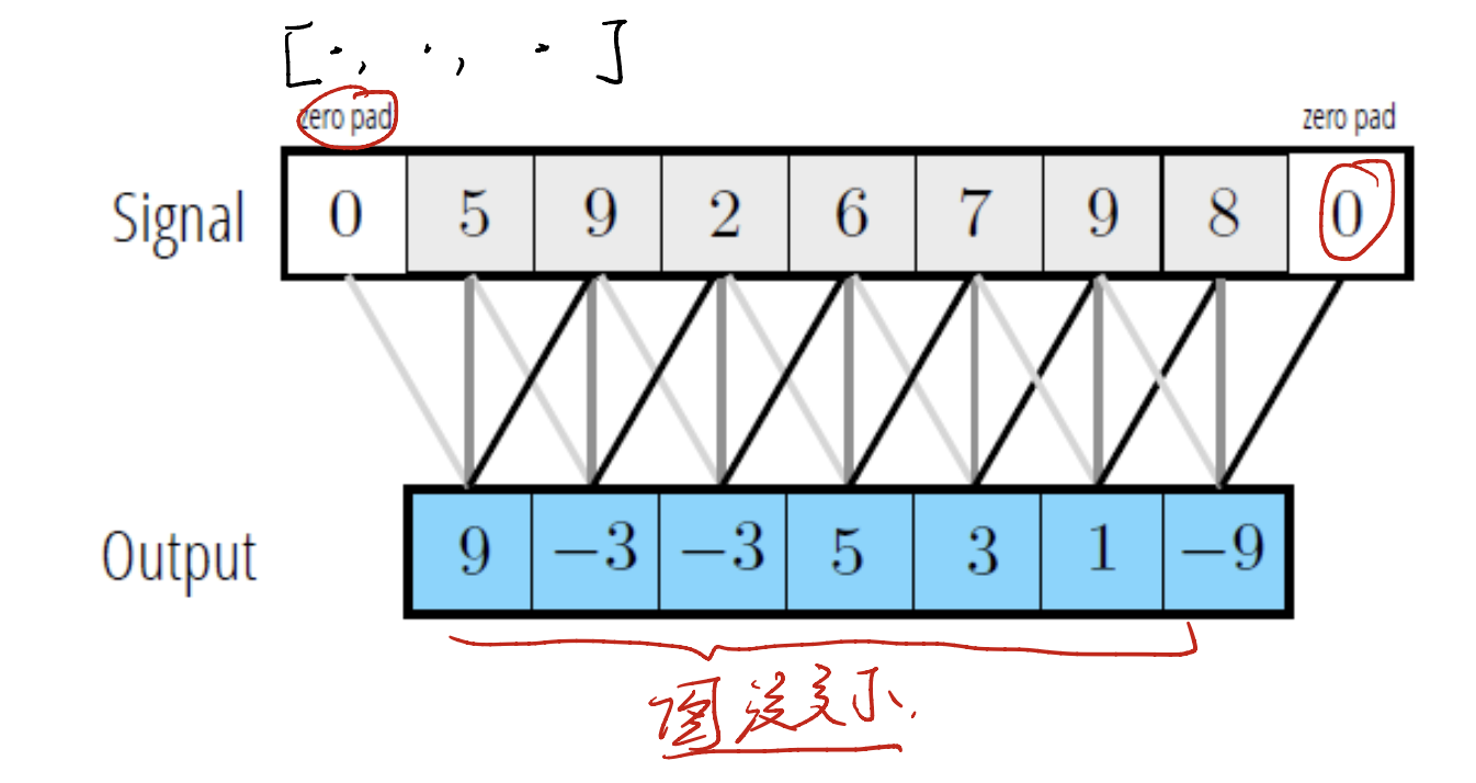
Just add some $0$ to the margin of the input image. When calculating it, it can maintain the output dimension.
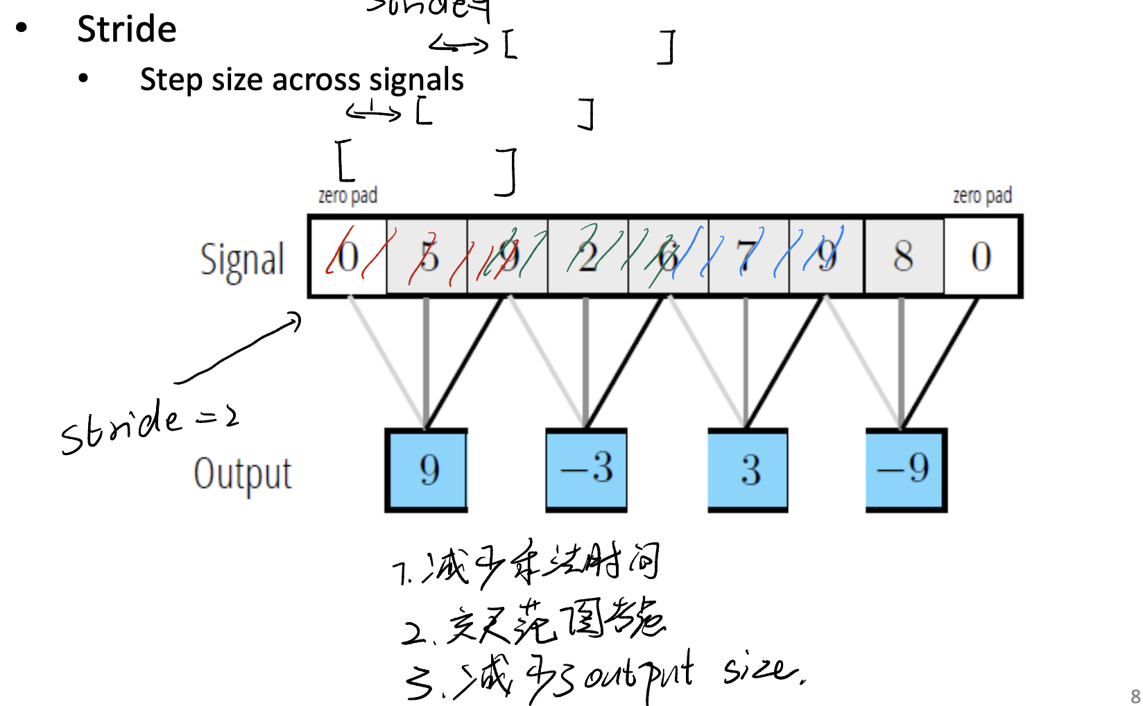
Trick 2: Stride
Stride likes the step of sliding. When our kernel scans through the whole picture, we can set the step for its moving.
The idea of stride is, the picture is very wide and has a lot of pixels, the useful features may not appear everywhere, when we set stride, we can accelerate the training loop, while keeping the information as much as possible.
And, with this trick, we can reduce the output size. Even more, we can consider more features across more range of pictures.
Define kernel Size and Number
An important question for us is to define the kernel size and the number of kernels we use.
- For the number of kernels, it is a hyperparameter. Normally, more is better than less.
- What does kernel look like? Or how about the size of a kernel? This is just what we want to learn…
Nonlinearity of CNN
We often need to add some nonlinearity to our deep learning model, otherwise, deep is meaningless.
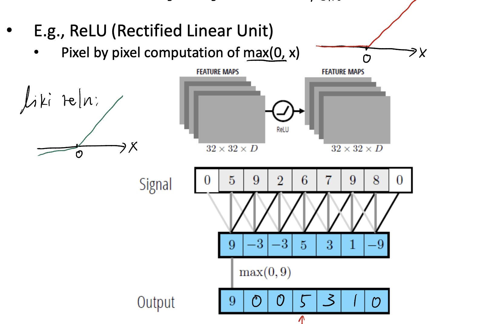
We often use Relu as our activation function.
Receptive Field
Receptive Field means the feature map “sees” how large the area is.
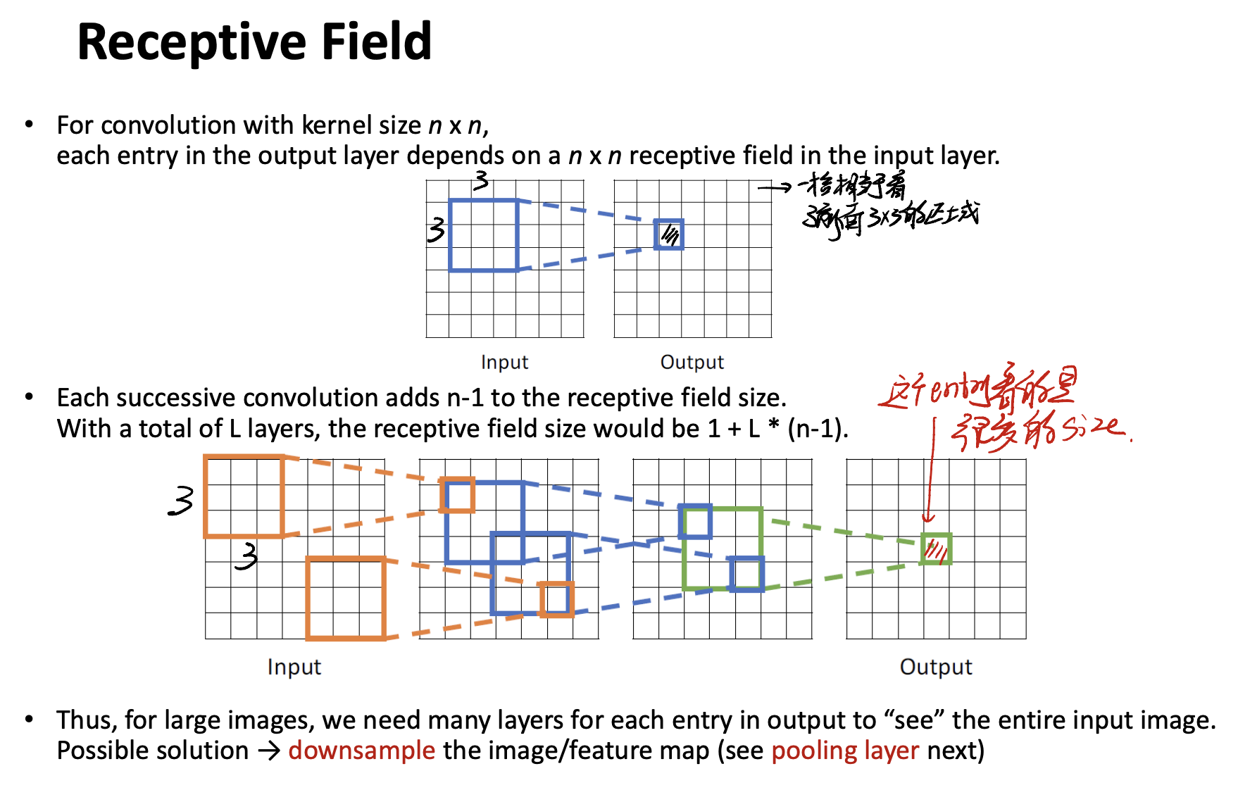
For example, see the pic above. One pixel in the output can “see” the original $3 \times 3$ field. This is receptive field.
For a deeper network, one pixel in the final output can “see” more and more regions of the input image. See the picture in the half-down part.
Receptive Field相当于说明一个pixel相当于看到了多大的原图。
A Variant of Convolution::Dilated Convolution
Now we introduce a variant of normal convolution, called Dilated Convolution.
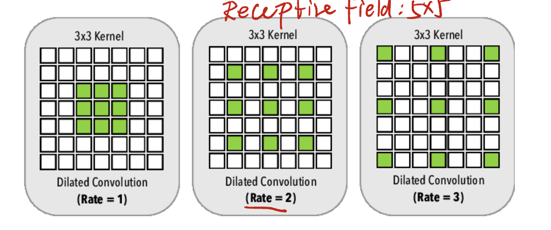
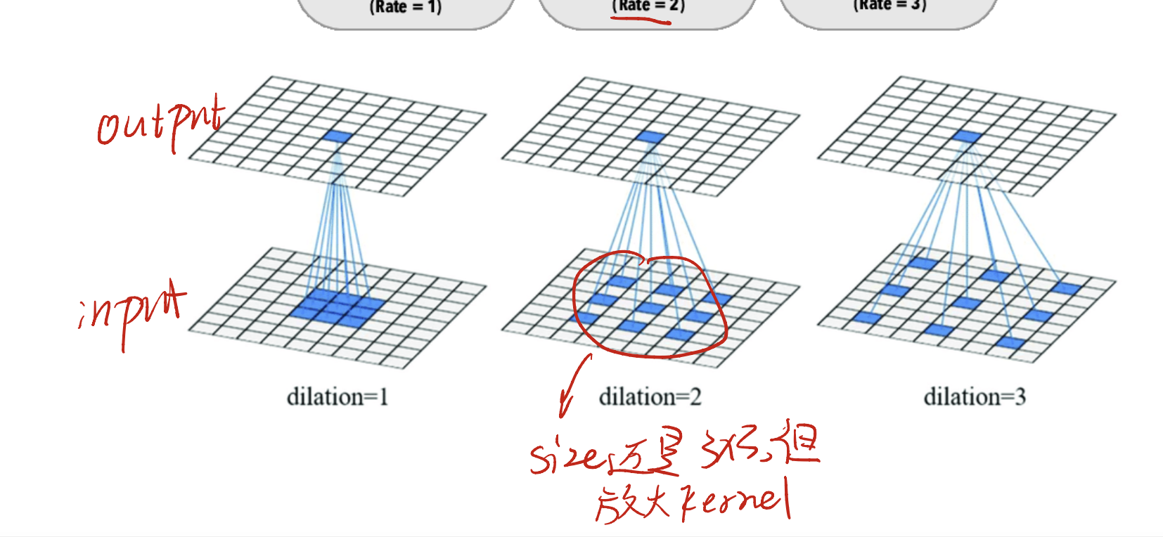
Let’s say that we have a $3 \times 3$ kernel. In a normal case, we can make a kernel like left side. 9 items squeeze each other.
However, in dilated convolution, we have a new hyperparameter called Rate. This is the margin of each element in the kernel. If we say that the rate is 2, it looks like the middle one; we say the rate is 3, it looks like the right one.
This Rate setting ensures that we can use the same size of kernel, to learn a wide range of features. In general, kernel in the same size but capable of handling a larger receptive field!
Pooling
The pooling layer is another useful layer in CNN.
Example of Using the Pooling Layer
Assume we want to detect a person. In one image, we may have multiple persons, some are large, others may be small.
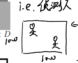
Let’s say we have two people to detect. And we have a $10 \times 10$ kernel to do this operation. However, this kernel can only detect a small person! As with people going large, the kernel needs to go large too, so that the kernel can detect all useful information for a larger person.
With pooling (aka downsampling), we can use the same filter, but with a small calculation effort!
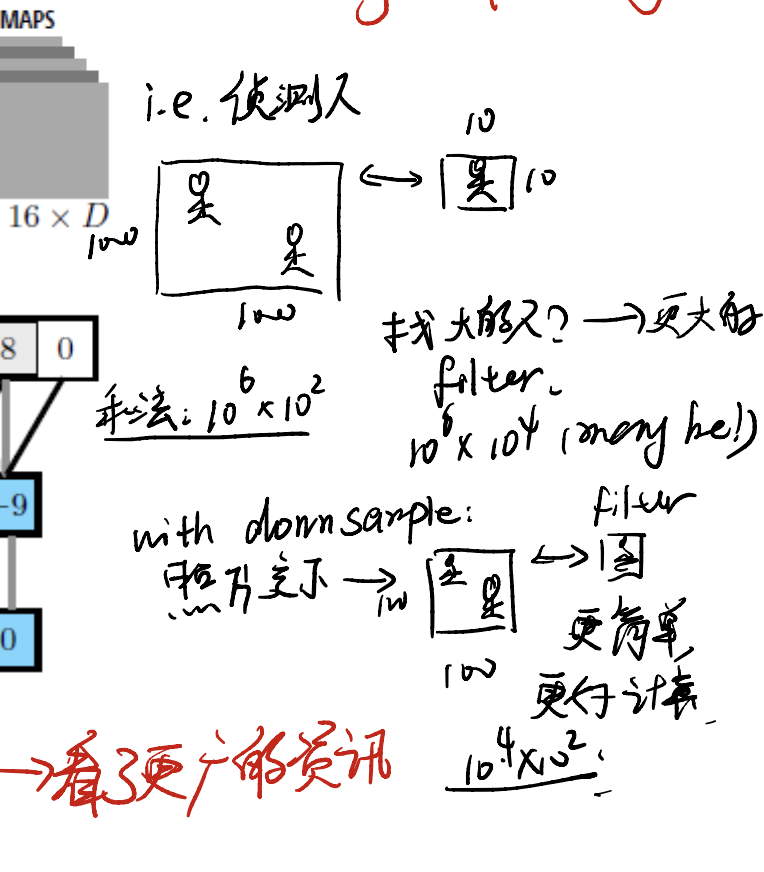
This is a trick which allows us to see more information contained in the image.
- Pooling can deal with dimension-reduction questions.
- Also, pooling increases the probability that we extract high-level information, which is good for learning features.
- Pooling can reduce the spatial size and provide spatial invariance.
We often use Max Pooling and Average Pooling.
Last Part::Fully Connected (FC) Layer in CNN
Final in final, we need to classify! This means we need a Fully Connected Layer to deal with our information. Let’s see.
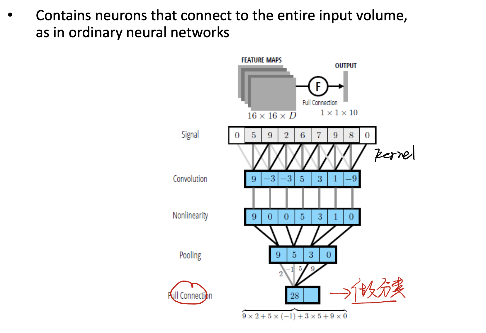
After convolution, nonlinearity, pooling… We finally get to the Fully Connected Network.
As we use all sorts of methods to reduce the dimension, we can now just use not so more parameters to get the final FC network.
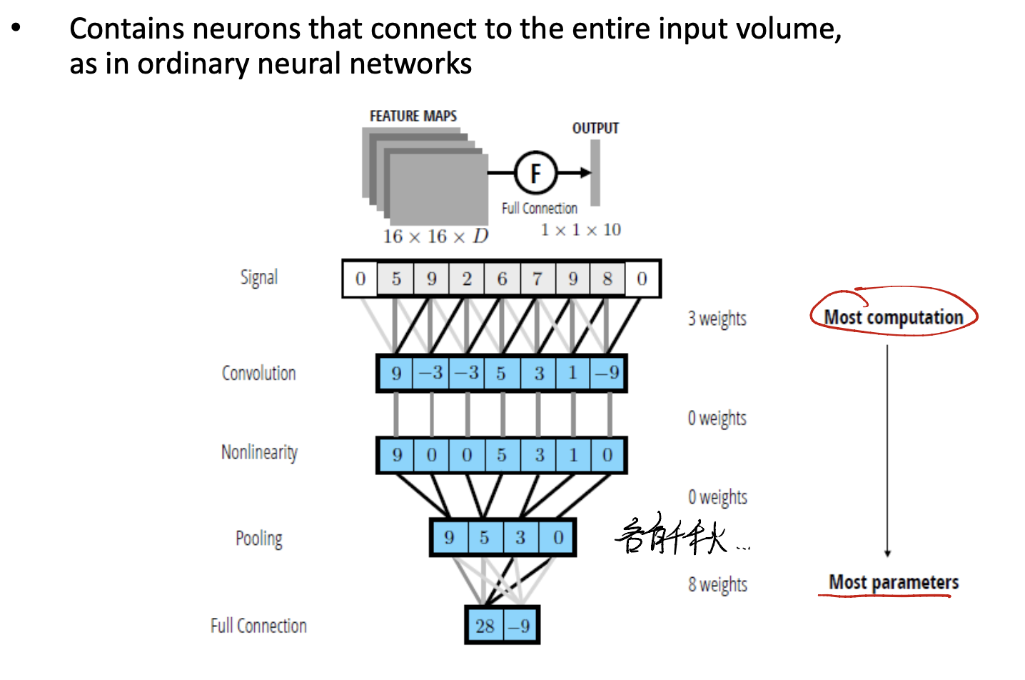
So this is the final!
Look Back of CNN
All Sorts of CNN
LeNet
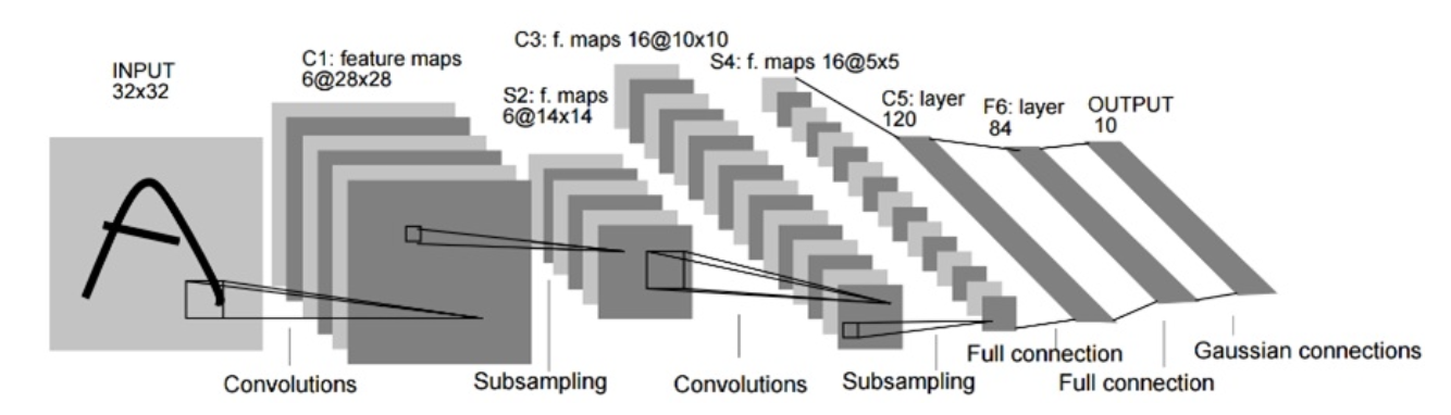
LeNet is the first architecture of CNN.
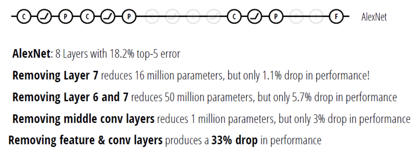
AlexNet
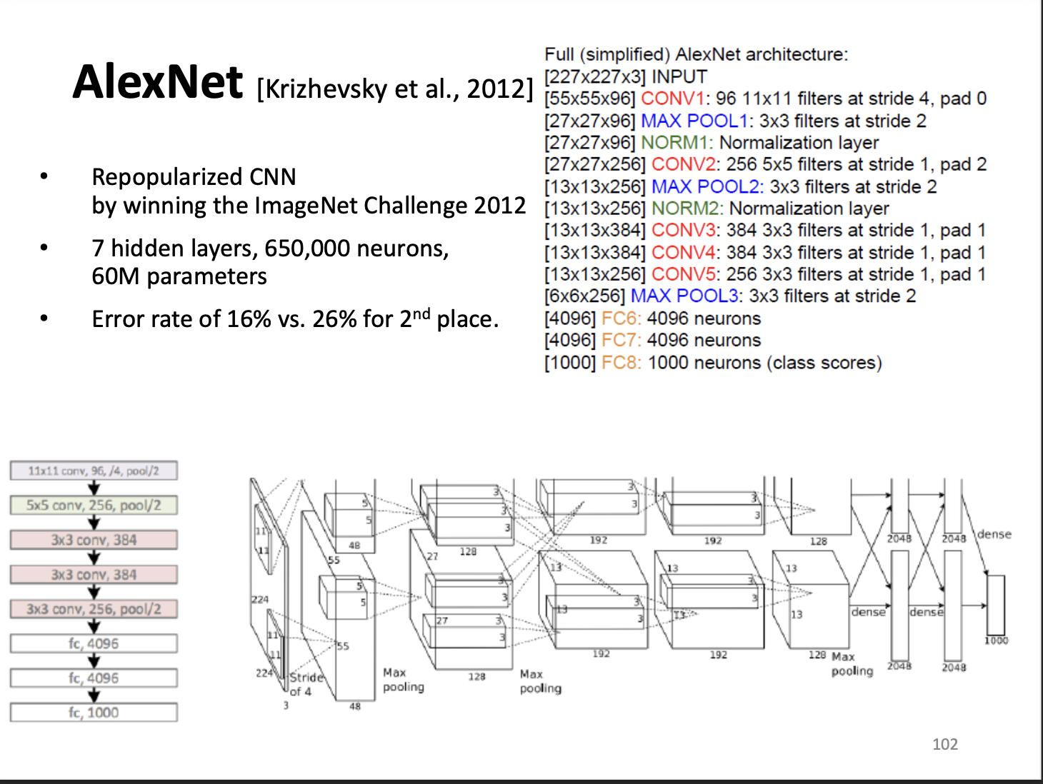
The AlexNet is a deeper vision. It proved that the Depth of the network is critical for performance.