Deep Learning for Computer Vision Lecture 3

2022 Deep Learning and Computer Vision Lecture 3

In this lecture, we will continue to go through CNN and its applications. Moreover, we will delve into other tricks and designs that increase the performance of CNN.

Recap of CNN

Firstly, let’s do the recap for CNN.

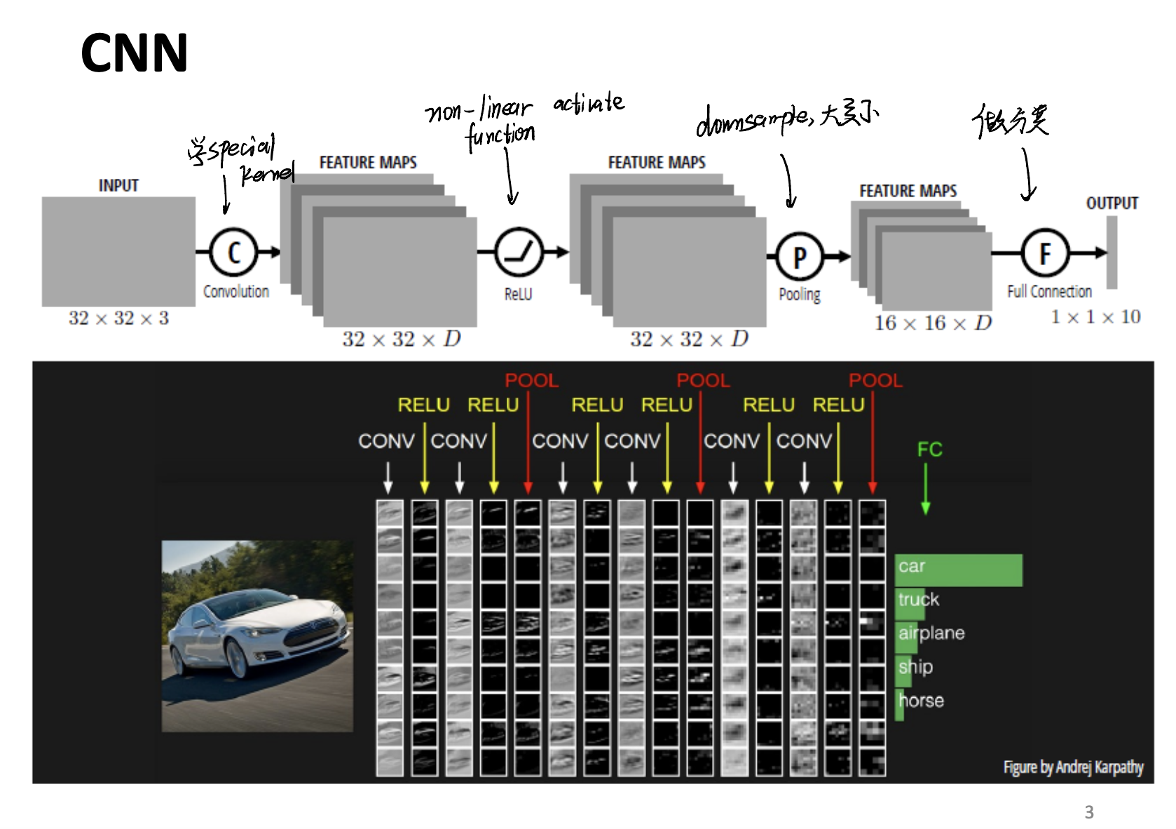
In general, there exists 4 steps of a training loop:

• Convolution - Using kernels to conpute the convolution. Kernels will learn what feature is in the image.
• ReLU - Activation function part. This will add extra non-linear parts in the CNN model.
• Downsampling - Polling part. Use for dimension reduction.
• Full Connection Neural Network - Use for image classification.

FC Layer

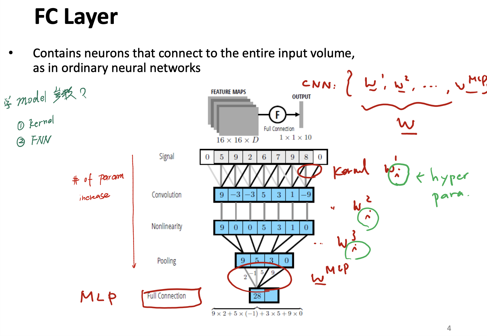
Full Connection layer, also known as MLP layer.

• From Signal $\rightarrow$ Convolution $\rightarrow$ Nonliearity $\rightarrow$ Pooling $\rightarrow$ MLP, the # of parameter is increasing.
• From Signal $\rightarrow$ Convolution $\rightarrow$ Nonliearity $\rightarrow$ Pooling $\rightarrow$ MLP, the conputation of model is decreasing.

All Sorts of Convolutional Neural Network

LeNet

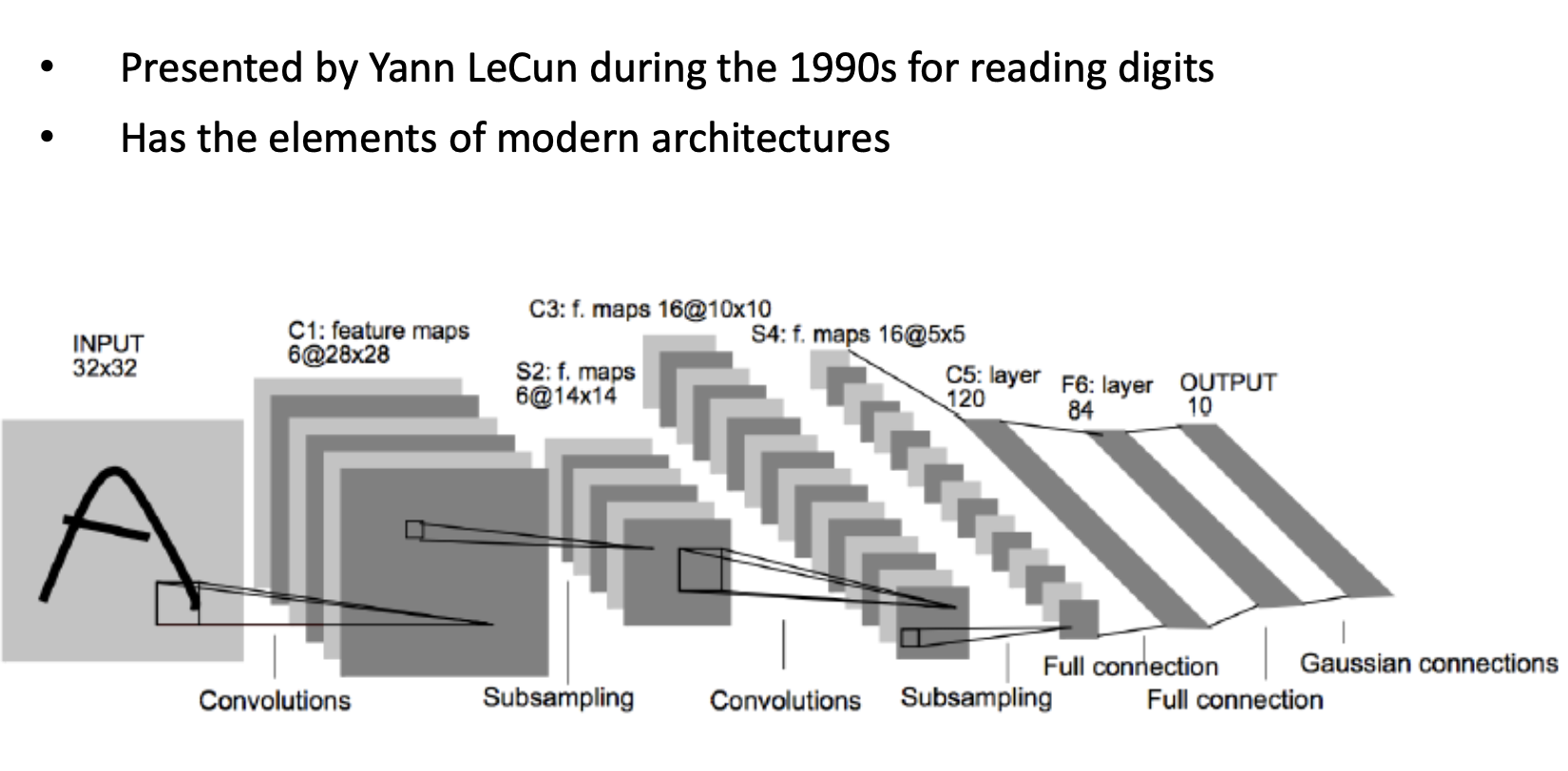
LeNet is a simple, initiative CNN.

AlexNet

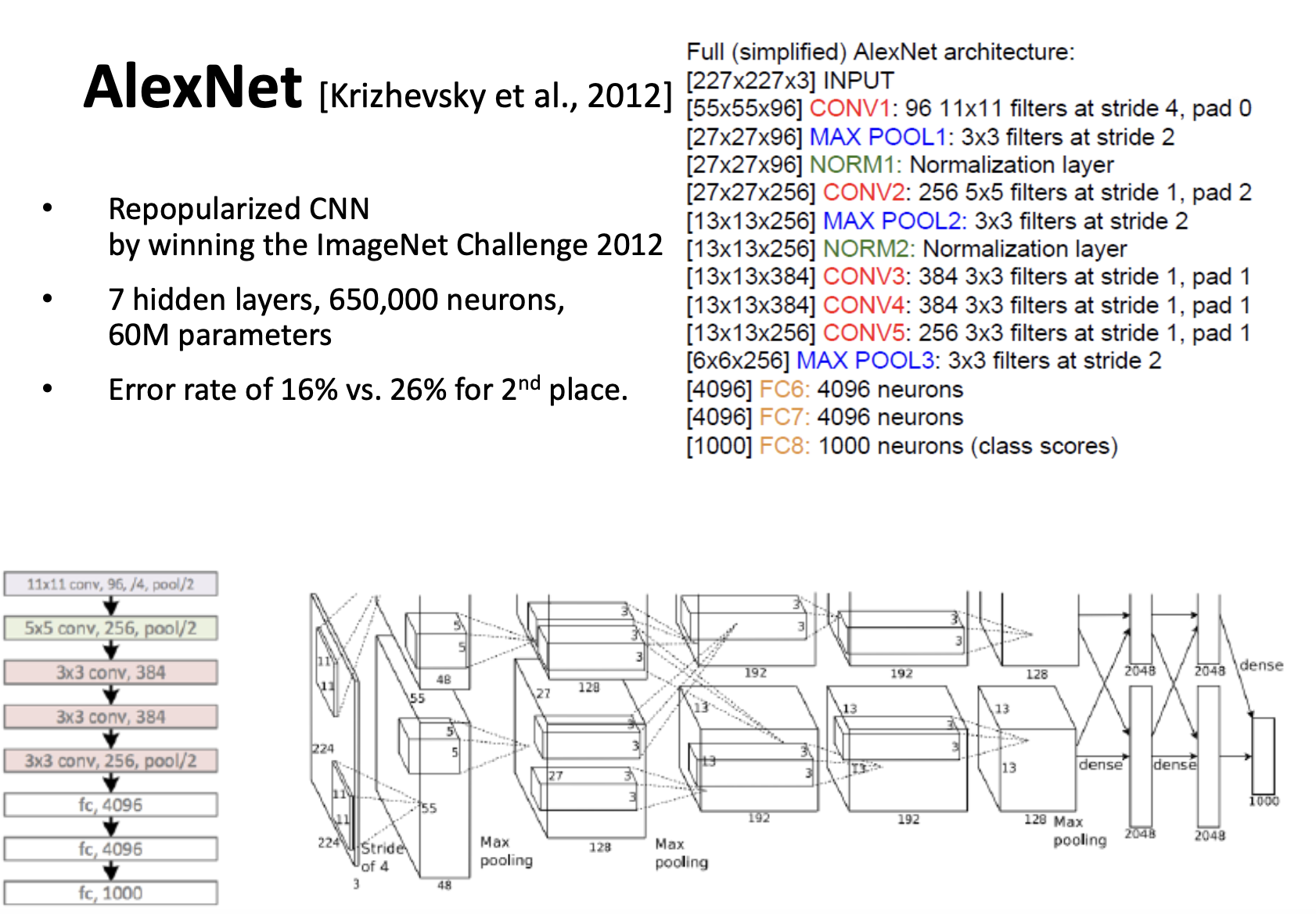
AlexNet is a kind of upgrade from LeNet. Let’s see the # of Hyperparameters in AlexNet.

Assume that:

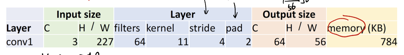
Say that the input size is $(227 \times 227 \times 3)$, and the kernel size is $11 \times 11$, we have $64$ kernels.

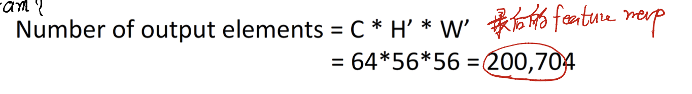
it is clear that the number of output elements will be huge. So here comes the question…

Deep or not?

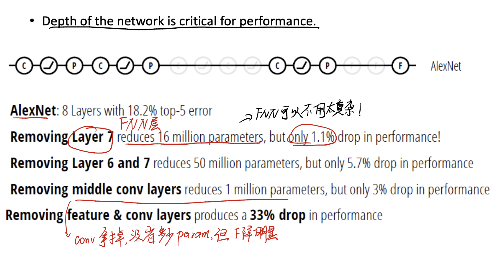
A huge amount of experiments shows that,

• If remove the convolutional layer, it will occur a significant performence decreasing.
• However, If we remove the MLC layer (fully neural network), the performence will not decrease a lot.

This tells us that the FNN do not need to be so complicated.

Trick1: $1 \times 1$ Convolution

In our mind, the kernel size must be at least $2 \times 2$. How about an $1 \times 1$ kernel?

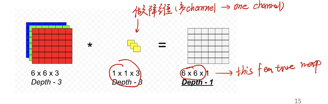
Obviously, using $1 \times 1$ kernel size can help us do the dimension reduction. See picture above.

Moreover, with activate function, we can add non-linear part into the feature map.

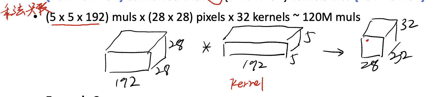
Example1: without $1 \times 1$ convolution

Assume we have feature image $(28 \times 28 \times 192)$. And 32 kernels with $(5 \times 5 \times 192)$.

Our calculation looks like:

Example2: with $1 \times 1$ Convolution

We always want to transform $(28 \times 28 \times 192)$ to $(28 \times 28 \times 32)$. Now we use $1 \times 1$ kernel.

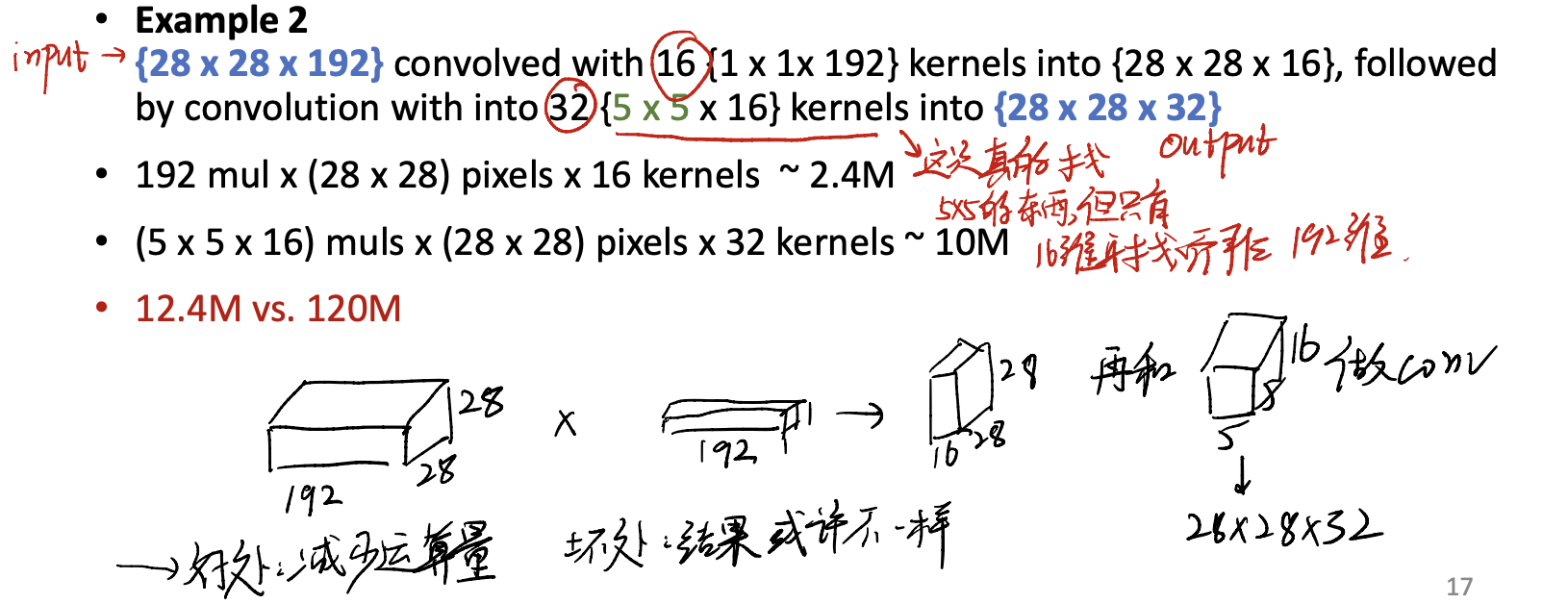
Pros and Cons

• Pros:
  • Reduce the computation extremely. (2.4M comparing to 10M)
• Cons:
  • You may get different outcomes each time.

ResNet

We know that it is an increasing layers game. But, can we just accumulate the layers back and forth? See.

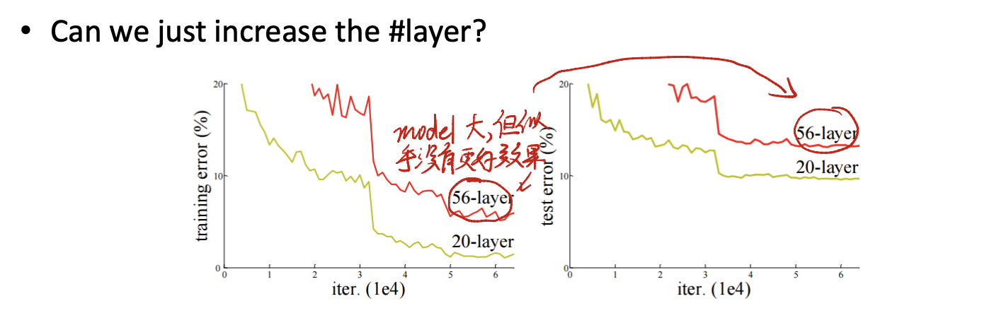
Comparing 56-layer to 20-layer, the model becomes larger than before, but we can not increase the performance. On contrary, it enlarges the test error.

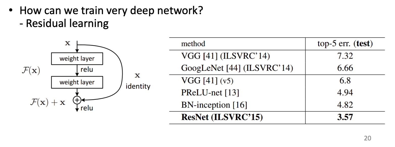
Our trick is:

• Jump off the block - comparing to original fully connected blocks, now we allow some input directly jump off some layers, till next layer. ( This is so called residual. )

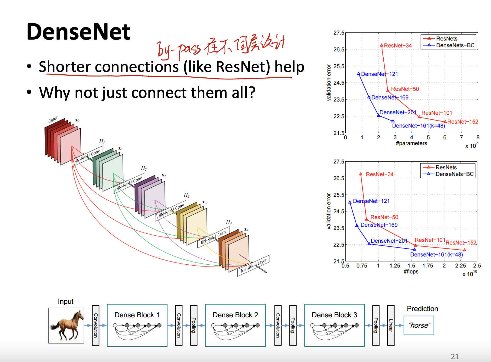
DenseNet

Google Net

Google Net focuses on efficiency and downsample the input.

Inception Module

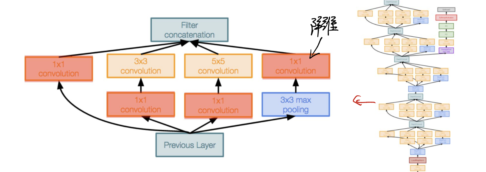
The goal of inception module includes,

• Parallel branches load - when computing, the module can parallelly load units.
• Calculate multiple times.
• Reduce channel dimensions - Use $1 \times 1$ layers to reduce the dimension.

Trick2: Global Average Pooling

Through global average pooling, a network can avoid large FC layers.

Trick3: Auxiliary Classifier

Use auxiliary classifier, the network can provide training guidance in an epoch.

Tranditionally, the model will know the loss value after the whole epoch finished. However, auxiliary classifier let the model know the loss during training loops.

相当于让model在training的过程中，知道模型学的怎么样，从而使模型更加容易收敛。

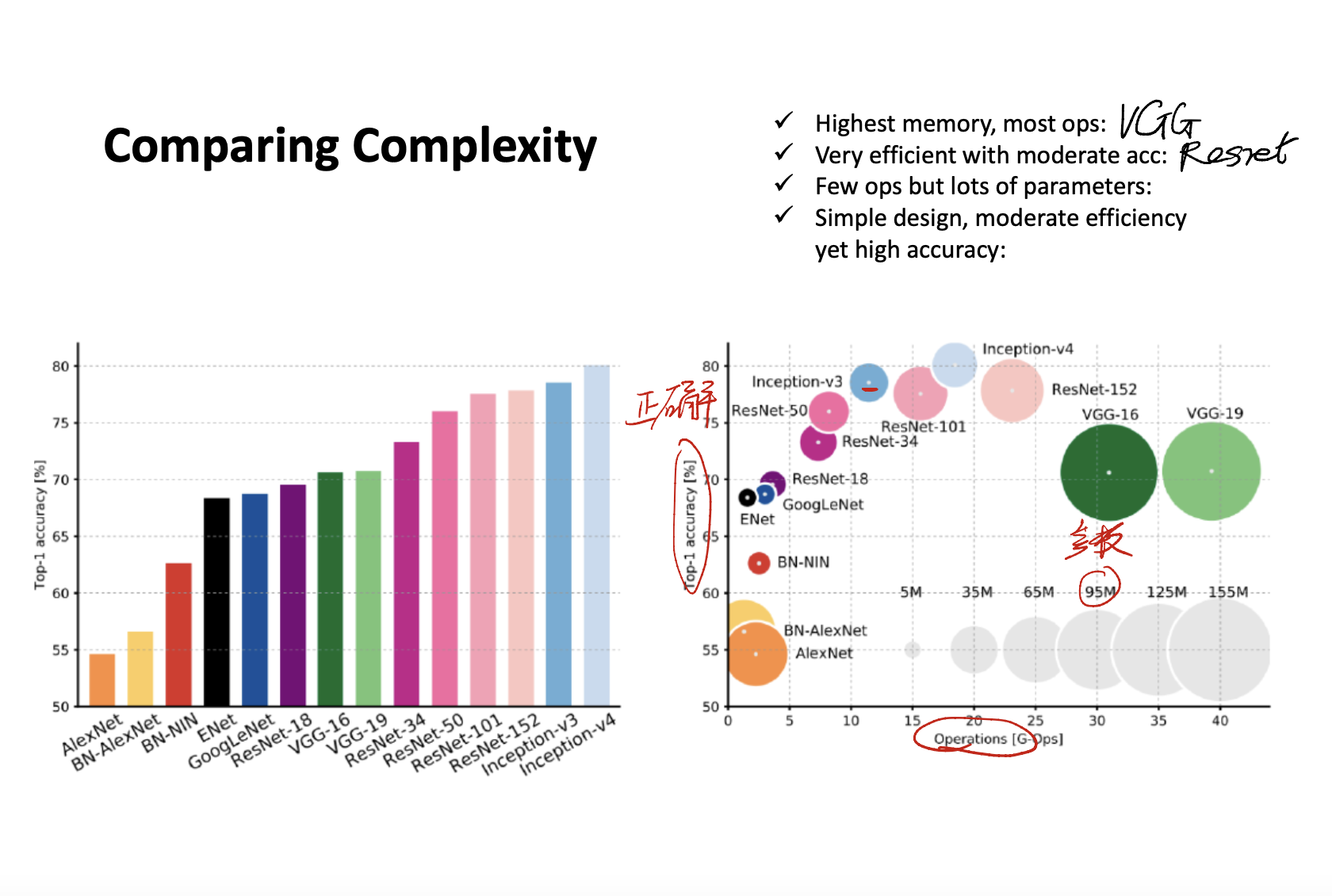
Model Comparison

Training Convolutional Neural Network

Sometimes it is really hard training the neural network. We need to delve into the details for training.

Generally, there are four ingredient in training. Includes,

• Backpropagation + SGD with momentum.
• Dropout
• Data augmentation
• Batch Normalization

Let’s see.

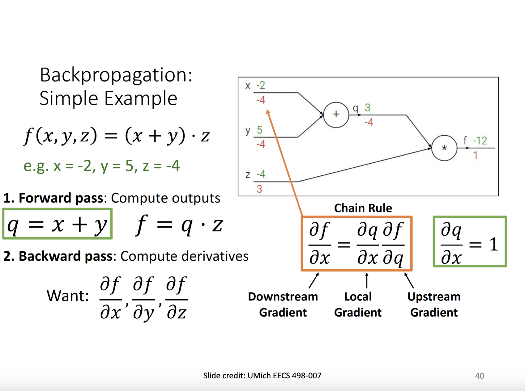
Backpropagation

Dropout

Dropout is a little trick helping us to learn parameters rapidly.

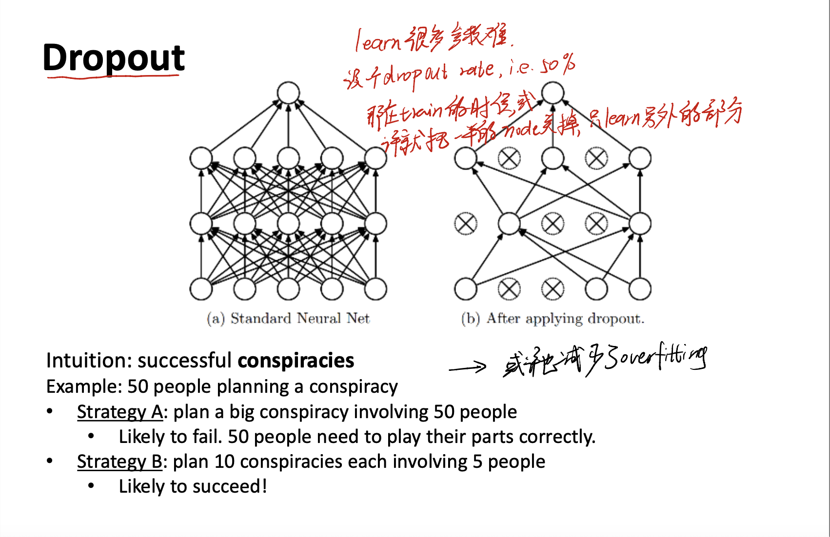
Let’s compare (a) and (b):

• (a) - we have the standard neural net with fully connected. This means that we have lots of parameters to learn. Costs lots of time and computation.
• (b) - We can set a dropout rate. i.e. 50%. When training, we can close 50% of nodes, just learning the remain part.

Formally, the main idea of dropout is - approximately combining exponentially many different neural network architectures efficiently.

The dropout method can reduce the # of parameters. Moreover, it may reduce the change of overfitting.

Data Augmentation (Jittering)

We may encounter the data set size problem. Collect a large amount of data is very hard! And, mark the label of each imgaes is also an expensive thing. What we can do is using the Data Augmentation method.

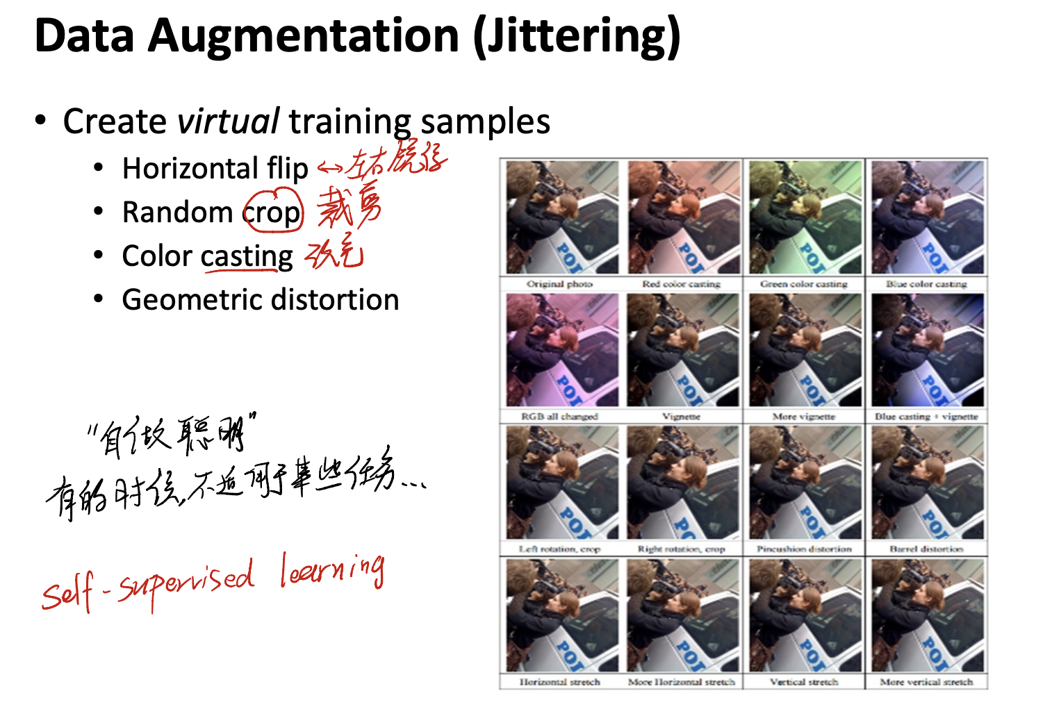
主要的方法有：

• Horizontal flip - 左右镜像image
• Random crop - 做裁剪
• Color casting - 改色调

但是，似乎也是一种自作聪明的方法。有的任务不适合用data augmentation。例如，假如在医学上，大部分人的心脏都在左侧。如果我们镜像这种图，machine会learn到一些很奇怪的表达，不适合我们的任务。

Batch Normalization

A very very important and useful method!

我们在训练中经常做Batch Training。即一次喂给我们的model一个batch的资讯。尽管我们会在分dataset时候做shuffle，但还是不能保证每一个batch都抽到差异不大的影像。我们希望找到办法，消除batch因为抽到的影像不同，从而影响learning的效果。

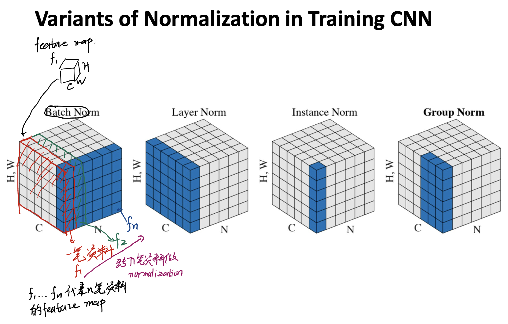
Generally, there are four types of normalization in training CNN.

上面的图中每一个cube都是一个feature map。

Case 1. Batch Norm

Image that our feature map is $C \times H \times W$. Where $C$ is the # of channels. And $H, W$ is the width and height of one feature map.

When doing Batch Norm we acturally do the normalizaton cross $n$​ data. Just like the blue area we marked.

简单而言，Batch Norm减少了不同feature map slice之间的差异。

Case 2. Layer Norm

Layer Norm更加简单一些，是在同一个feature map中来做normalization，减少的是feature map slice内的差异。

Case 3. Instance Norm

针对单独一笔资料来做normalization。

Case 4. Group Norm

根据使用者的设定来做normalization。

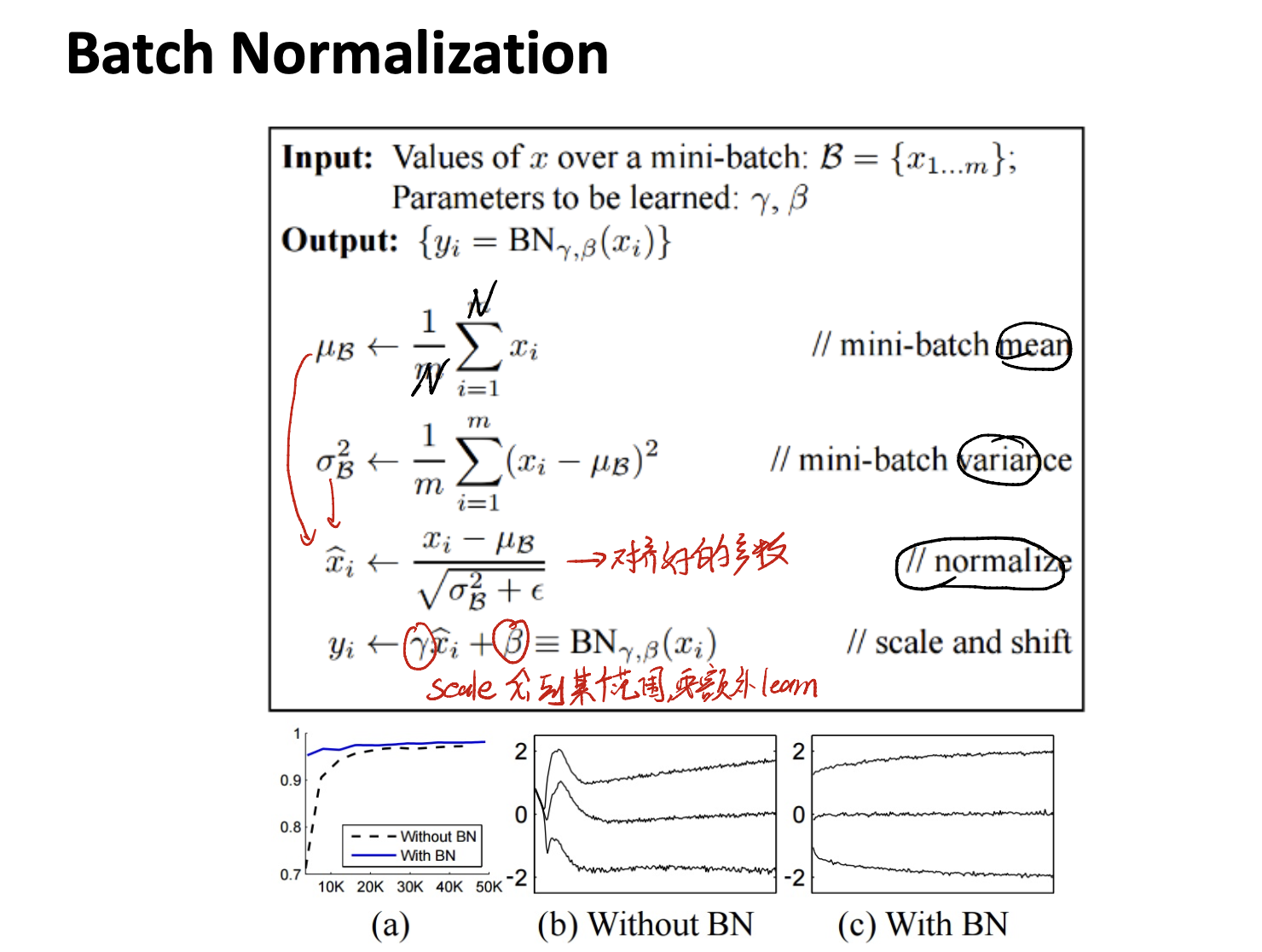
Batch Normalization Algorithm

Remark of Batch Normalization

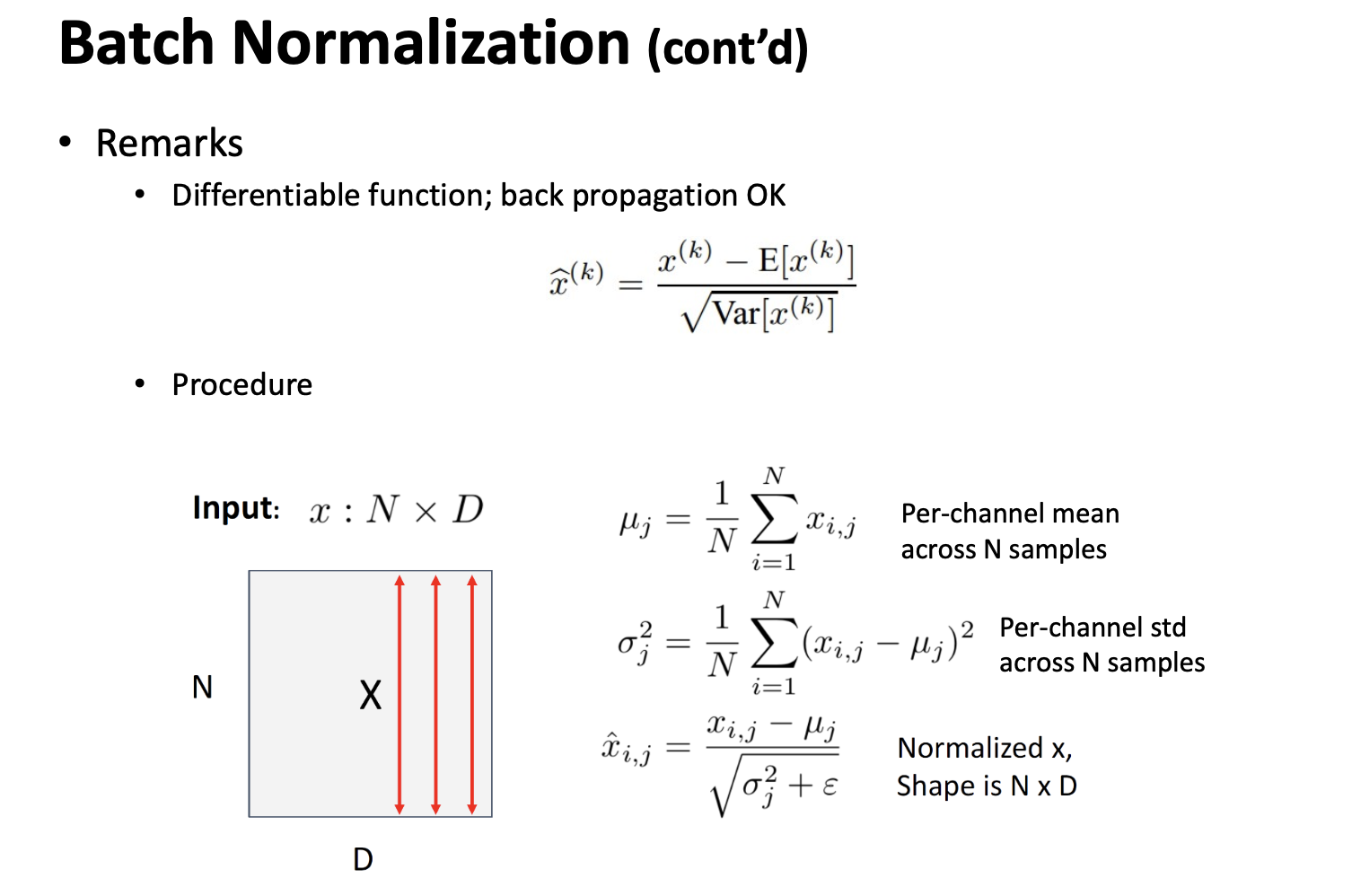
Procedure of Batch Normalization

Image we have the input with dimension $N \times D$. Where $N$ is the # of samples in one batch, and $D$ is the dimension of one feature map, aka, $C \times H \times W$. Generally, we do the normalization on one channel.

Calculate the per-channel mean across $N$ samples:

\[\mu_j = \frac {1} {N} \sum_{i = 1}^N x_{i, j}\]

Calculate the Per-channel standard deviation $\sigma_j^2$:

\[\sigma_j^2 = \frac {1} {N} \sum_{i = 1}^N (x_{i, j} - \mu_j)^2\]

Finally do the normalization part.

Mind that the batch normalization must be done on both training and testing part.

In testing, we do not have the batch. In this case, we can record the $\sigma$ and $\mu$ in training part, and directly use them in testing part.

In CNN…

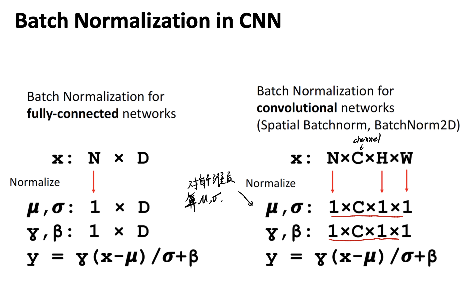
在CNN中，我们是对每个维度算$\mu, \sigma$，最后跨channel进行操作。

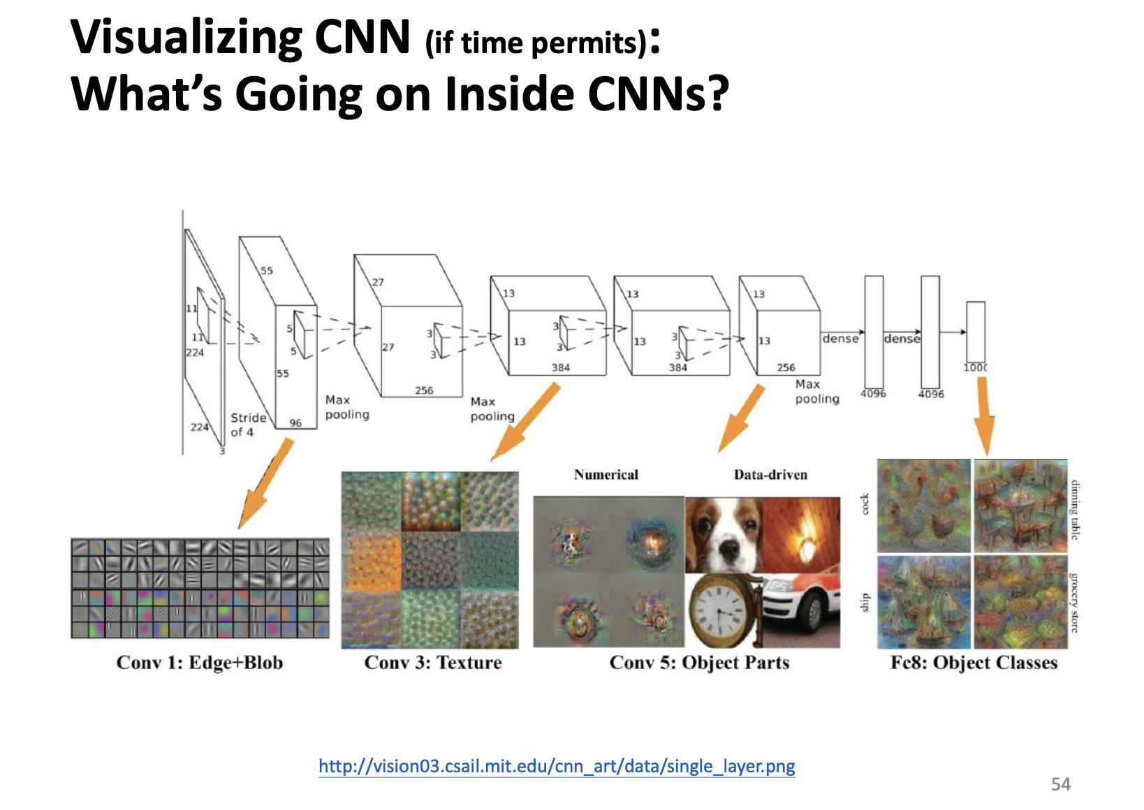
Visualization of CNN

To avoid so called black box. We want to visualize the CNN kernel. To see what it leart?

We always want to visualize the final layer of CNN. With respect to PCA, t-SNE, and so on.

t-SNE Method

We often use t-SNE method to do the visualization. The reason is,

• Powerful tool for data visualization.
• Help understand black-box algorithms like CNN.
• Alleviate crowding problem.

Other layers?

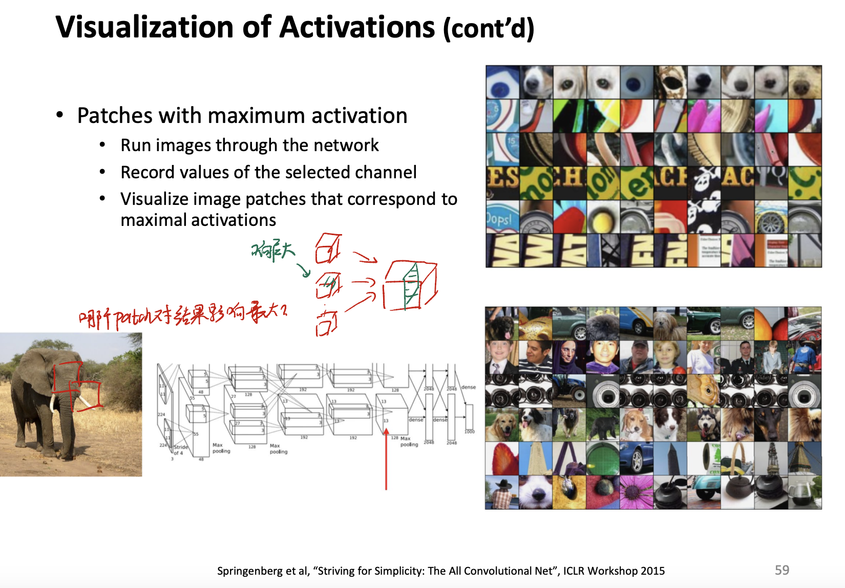
In other layers, we are more interested in the maximum activation problem. To get the feature picture, we can do:

• Run images through the network or the layer,
• Record values of each selected channel. (Mind that we can only do it on channel. A channel is connected to a kernel, so that we can find which part of the image reacts a lot.)
• Visualize image patches that correspond to maximal activations.

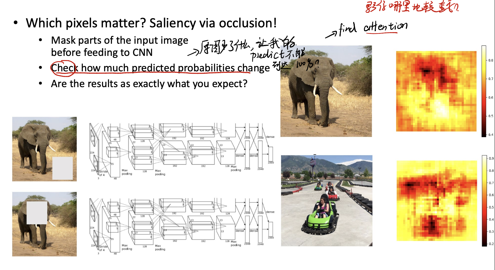
Saliency with occlusion…

可以通过mask部分image的方式来找到最重要的部分。这也相当于让我们知道kernel识别到了影像的什么位置，从而导致能够识别并classify某个image。

Activation maximization

Activation maximization is a technique that helping us find the most critical part in a layer. The idea of activation maximization is,

\[x^* = \arg \max_{x, s.t. ||x|| = \rho} h_{ij}(\theta, x)\]

where $x$ is our input, it usually can be a random noise. $\theta$ is our trained model parameter. we must make sure that it is fixed. And $h_{ij}$ is the activation of a given unit $i$, from a layer $j$ in the network.

After we get the random input, we can perform gradient ascent in the input space. To maximize the $h_{ij}$.

Moreover, we need to specify two hyper parameters: learning rate and stopping criterion.

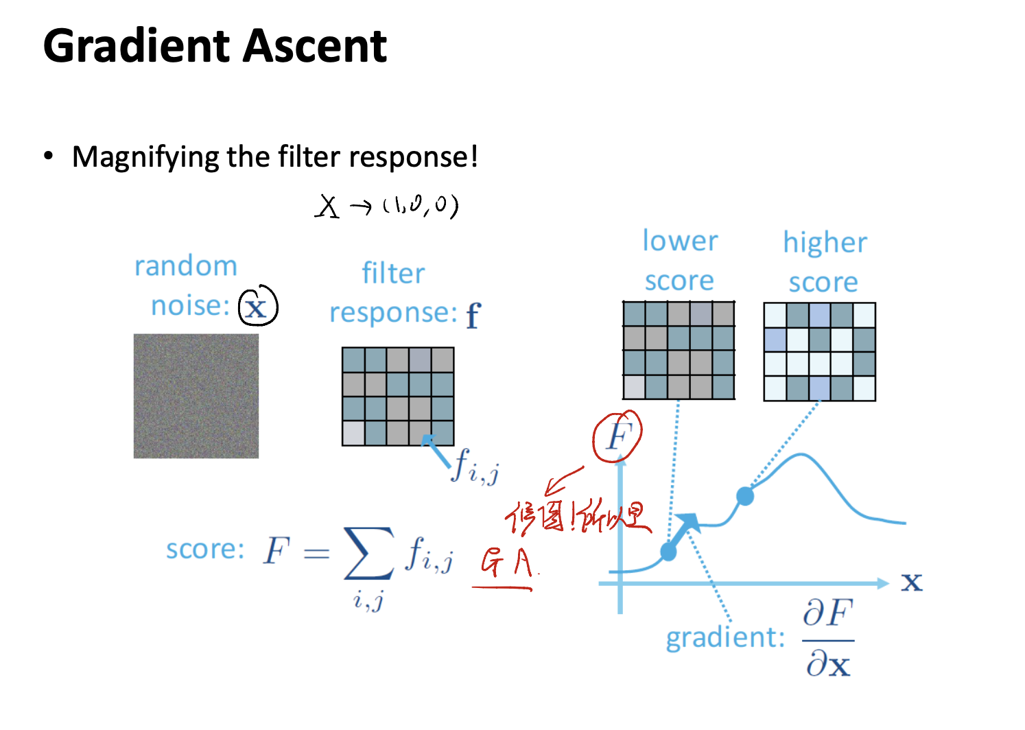
Image Segmentation

Now we introduce the next part of image classification, which is, Image Segmentation.

In image segmentation, our goal is to group pixels into meaningful or perceptually similer regions.

What is “similar” pixel?

i.e. colour, meaning, brightness, etc.

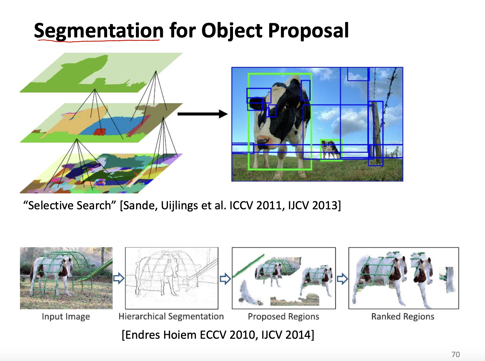
One of the application of image segmentation is object detection. See:

More Tasks in Segmentation

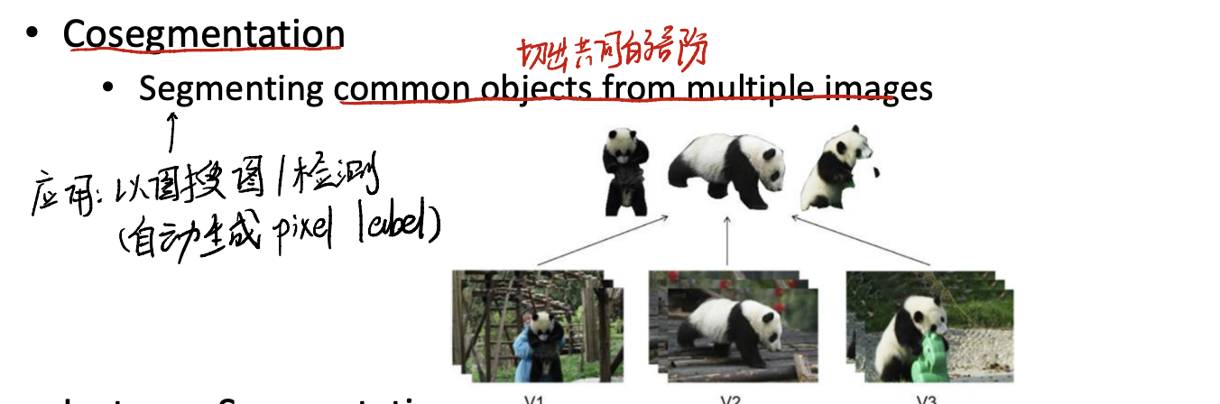
• Cosegmentation

Cosecmentation is a technology that segmenting commom objects from multiple images.

常见的应用是“以图搜图”。

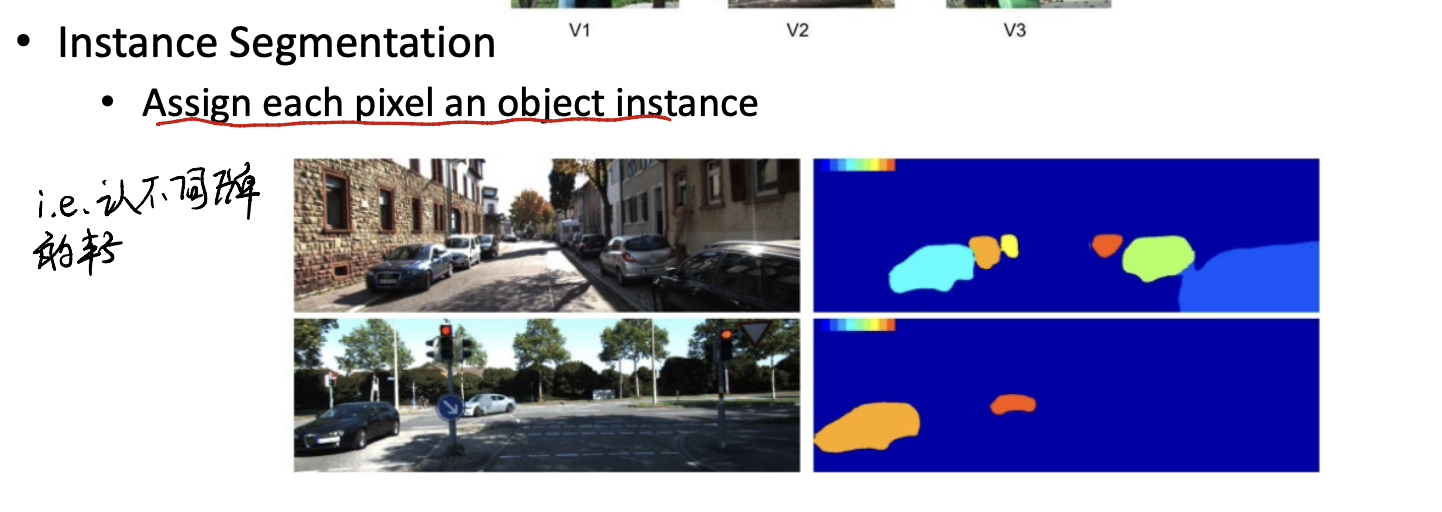
• Instance Segmentation

Instance segmentation aims to assign each pixel an object instance. i.e. figure out different type of cars.

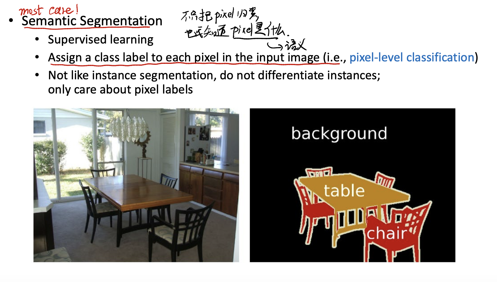
A Pratical Segmentation Task

Semantic Segmentation is one of a pratical segmentation tasks. It is a kind of supervised learning task. Not only categorised the pixels, but also need to assign a class label to each pixel input image.

However, it does not care difference instances of one object.

Sliding Window Method

One method is Sliding Window Method. In this method, we just use a CNN kernel, force it traverse all pixels in an image, and do the classification.

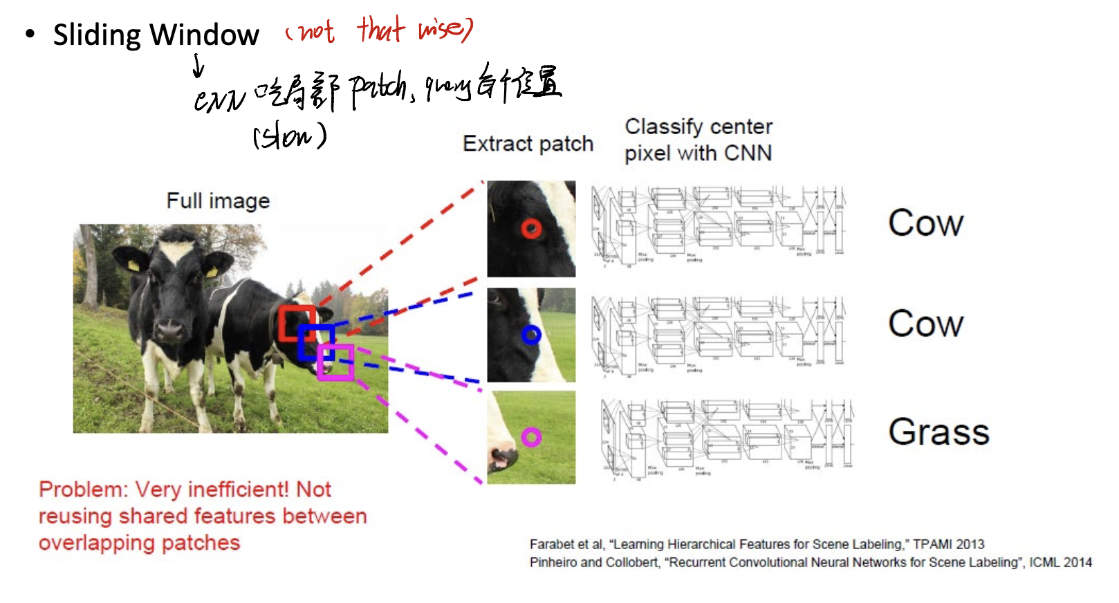
But it is not a wise method! See, the efficiency of this method is really slow, as we need to traverse all pixels! Many computations needed.

Fully Convolutional Nets

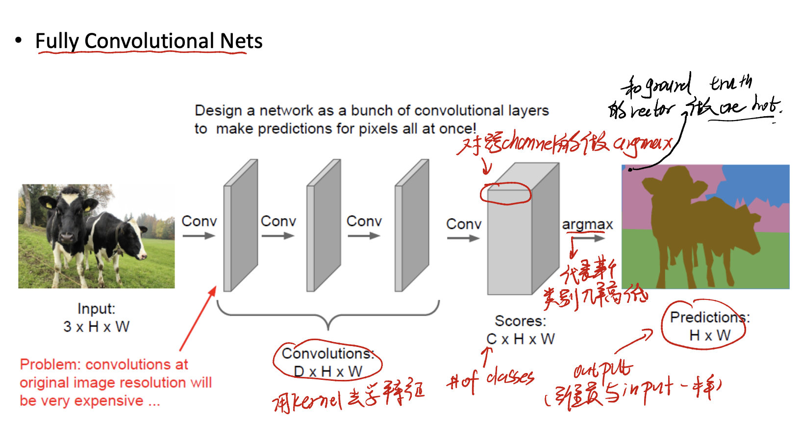
Another way is to use Fully Convolutional Nets. We use kernels to learn features, and form a wide feature map, with dimension $(C \times H \times W)$. Then, we do the $\arg\max$ onto the channel. To see what class a pixel is. Finanlly form the predictions with $(H \times W)$.

But it is also inefficiency! Improve it?

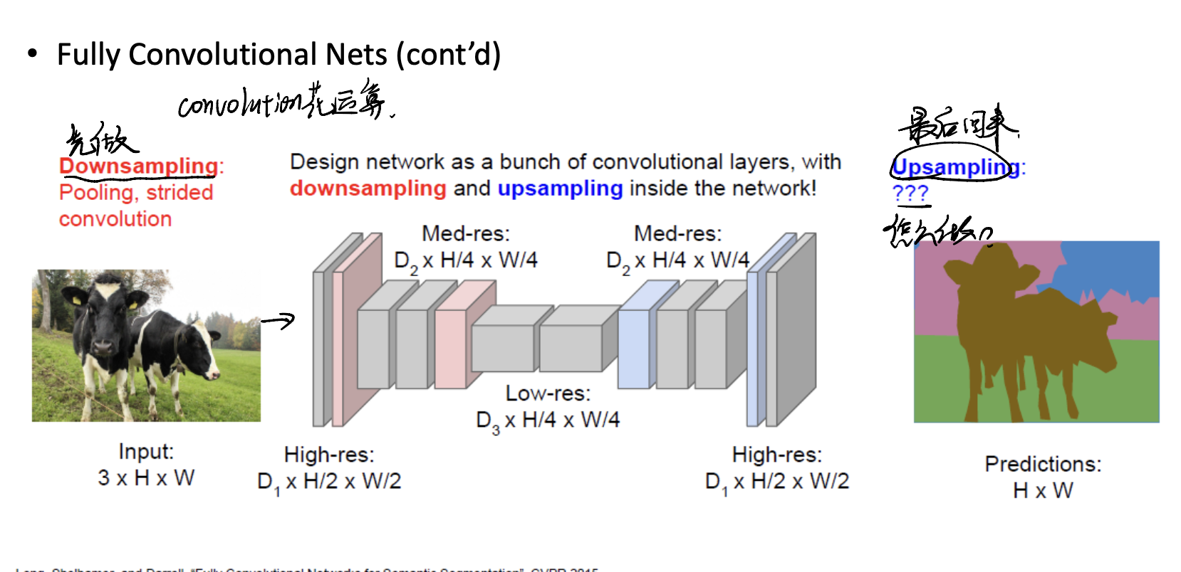
We can zip the image into a small one, and reconstruct it to the origional size.

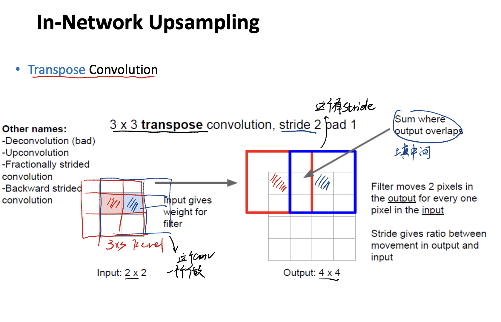
Let’s introduce the most important part: Upsampling.

Upsampling

Unpooling

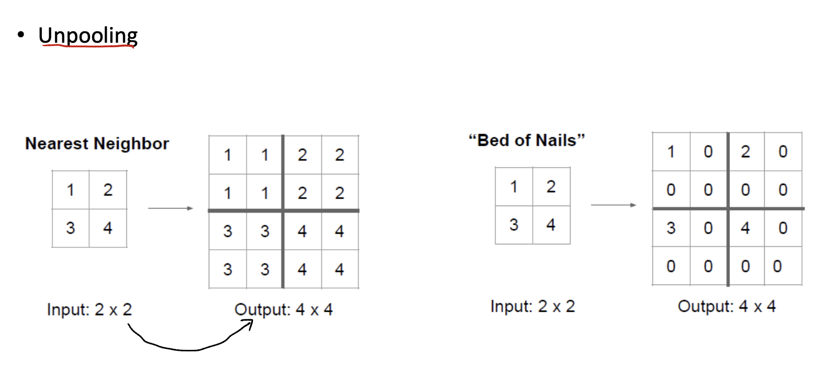
• Nearest Neighbour - 采用一样的value填充padding。
• Bed of Nails - 补0。

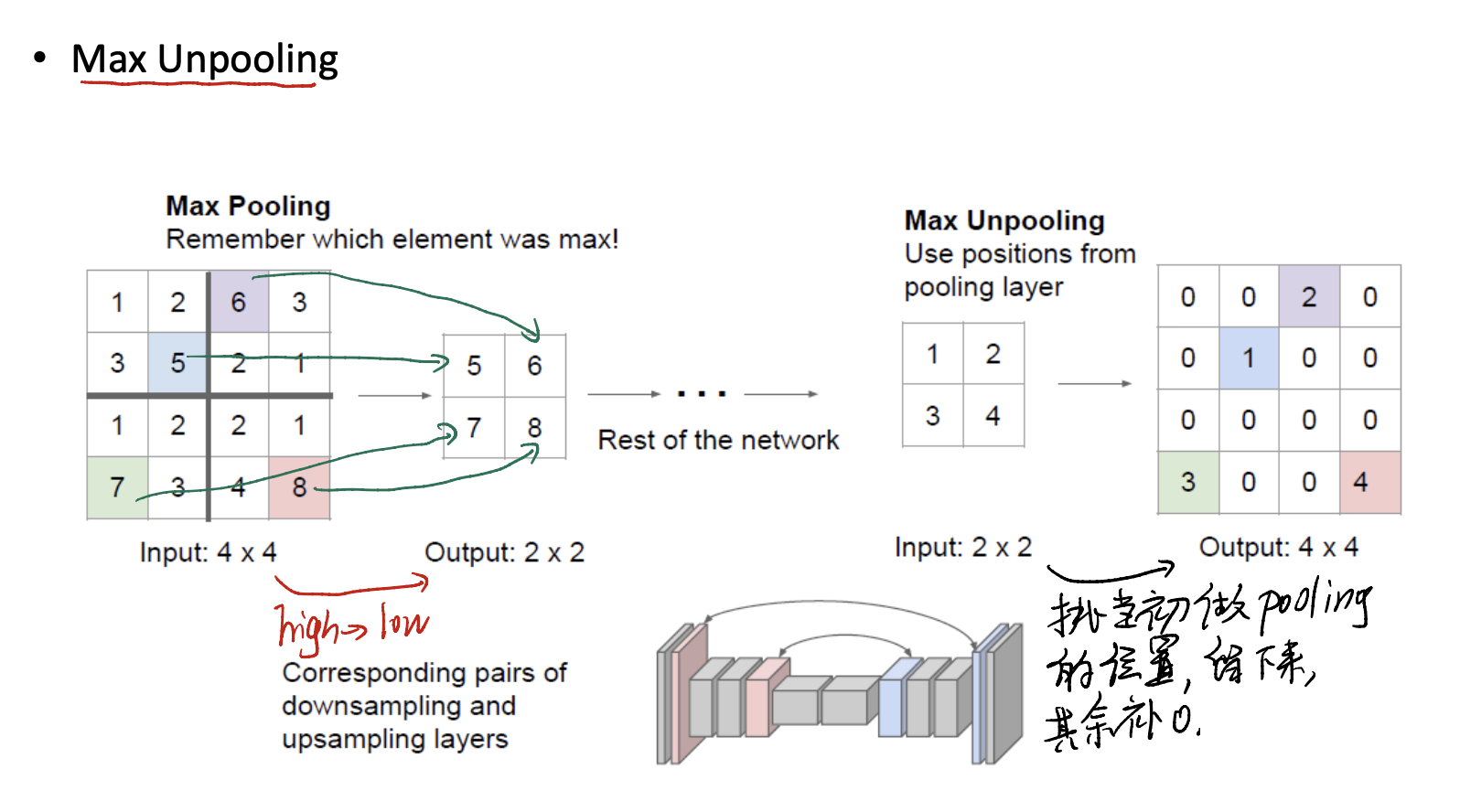
Max Unpooling是和Max Pooling相反的方法。

在Max Pooling中，我们记住了每个element的位置。所以在Max Unpooling中，我们要按照Max Pooling的位置进行element的还原，将这些填充到对应的区域，其他区域补0。

Learnable Upsampling

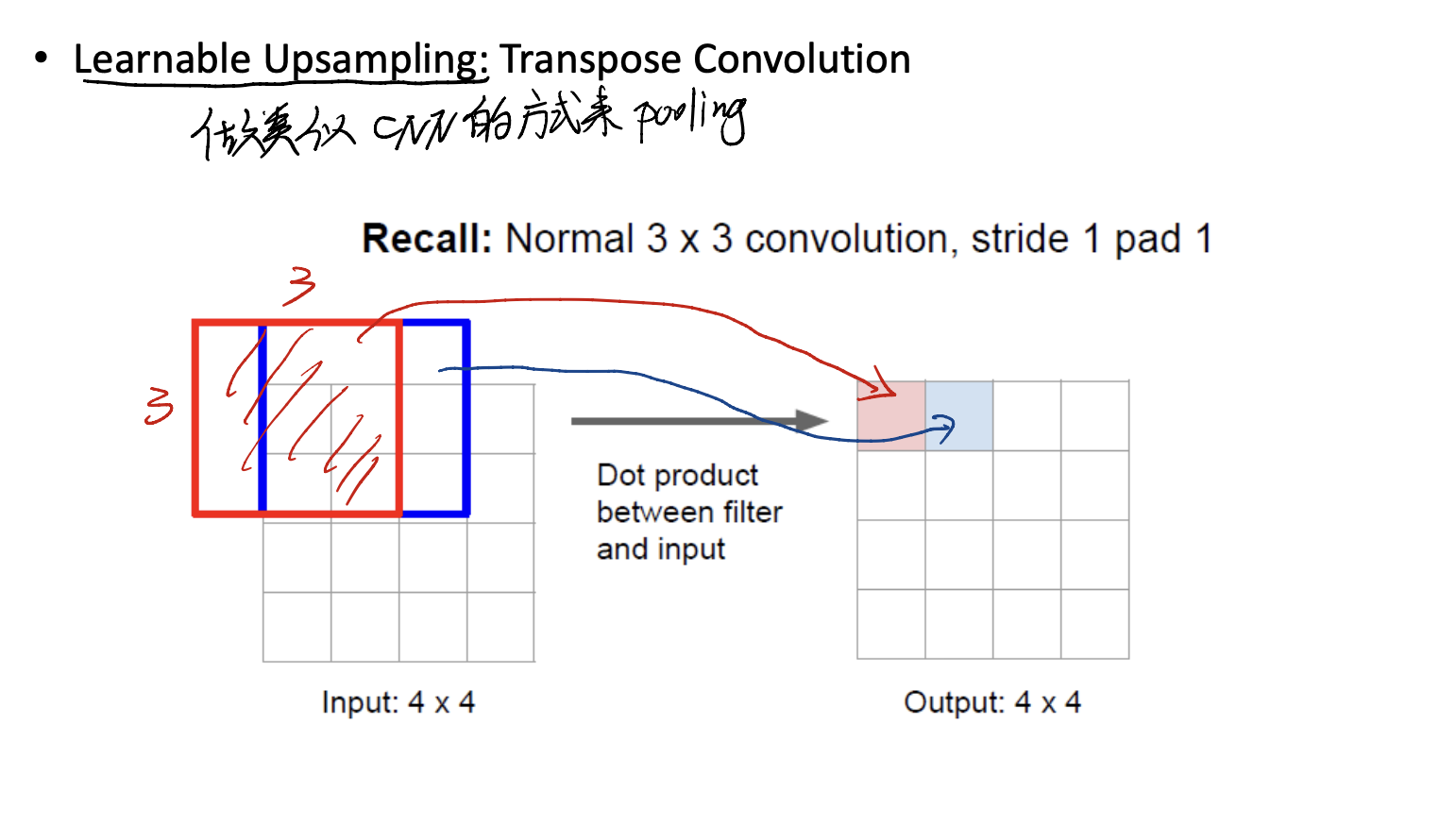
用类似CNN的方法来做，是一种learnable的方法。