Deep Learning for Computer Vision Lecture 1

2022 Deep Learning for Computer Vision Lecture1

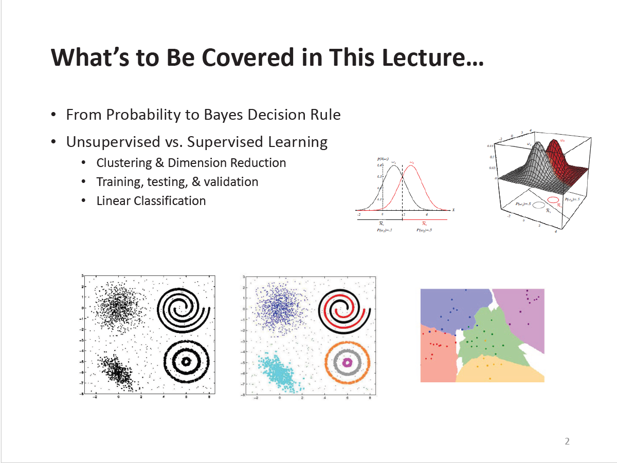
In this lecture, We shall review some basic machine learning concepts. And, some techniques.

Example: Testing of COVID-19

When testing of COVID-19, we will surely always meet positive/negative test results. And we of course can get two distribution of positive/negative results. The further away from each other, the better.

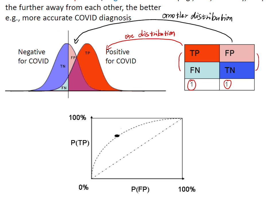
Mind that in case below, we get:

• One distribution is about TP(True Positive, aka “test right and surely right”) and FN(False Negative, aka “test wrong but surely right”). These two indicators are all connected with positive for COVID distribution.
• Another distribution is about Negative for COVID. One is FP(False Positive, “test false but surely true”), another is TN(True Negative, “test the people do not get COVID, and in fact so do him/her”).

Bayesian Decision Theory

Now we shall talk about Bayesian Decision Theory. This is the pivot of our decision system. First and foremost, let’s take a classification/detection task as our example.

Assume we have a 2-class classification task. See if a student would pass or fail the course of DLCV, with a probabilistic variable $\omega$. ($\omega = \omega_1$ for pass, and $\omega = \omega_2$ for fail)

Prior Probability

A priority or prior probability reflects the knowledge of how likely we expect a certain state of nature before observation.

For example, we have $P(\omega = \omega_1)$. This can be the prior probability that the next student would pass DLCV course.

即，在没有其他information的情况下，只来修课，pass这一门课的机率。

And the priors must exhibit exclusivity and exhaustivity. i.e.

\[\sum_{i = 1}^n P(\omega_i) = 1\]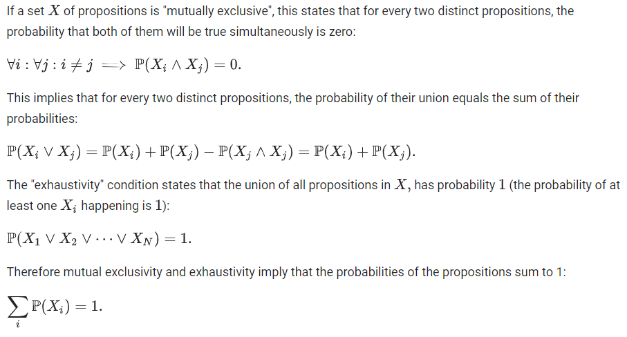

Decision rule based of priors only

有了先验机率，我们自然要想到办法做出判断，才能体现机率的价值。现在我们来看如何制定我们的Decision Rule呢？

可以这样想，假设我们期望$\omega_1$发生，那就最好要有：

\[P(\omega_1) > P(\omega_2)\]

否则我们认为$\omega_2$更容易发生。

这是一个很直观的规则，但更进一步，这个规则出错的机率是多少？好像priors并没有办法给我们答案。

Class-Conditional Probability Density

考虑到我们做的是分类问题，首先我们应该专注在分类的机率密度函数上。

所谓的probability density function(PDF)/class-conditional density，以上面的DLCV课程通过情况为例子，可以写成：

\[P(x | \omega_1)\]

这个式子是一个条件概率：在$\omega = \omega_1$的条件下观测。意味着我们这个概率针对的是通过的同学，希望知道通过的同学花费不同的学习时间$x$的概率是多少。

同样地，我们也要考察$\omega = \omega_2$的情况，即未通过的同学，他们所花费的学习时长是多少。

最后可以画出这种图像：

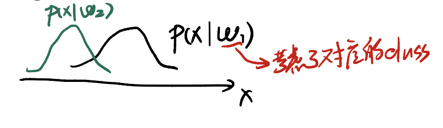
其中，$x$是学习时长。我们通过这种条件概率的PDF，能很好地把不同类别考虑进来，从而做出更加合理的推断。

Here’s (hopefully) the hypothetical class-conditional densities reflecting the time of the students spending on DLCV who eventually pass/fail this course.

Posterior Probability & Bayes Formula

现在问题到了这一步。如果我们知道了所谓的prior distribution和class-conditional density，我们又能怎样设计一个更加合理的decision rule呢？

Data we retrive before inference

在进行推断之前，我们拿到了两个数据：

• prior distribution: 即 $P(\omega_i)$ 。理解成去年同学的通过情况

• class-conditional density: 即 $P(x

  \omega_i)$ 。不同类型的同学所花费的学习时间

我们要推断的是，花多少学习时间，能变成$\omega_i$的状态？

Bayes Formula comes

首先我们来review一下Bayes Formula。它们是：

\[P(\omega_i, x) = P(x | \omega_i) P(\omega_i) = P(\omega_i | x) P(x)\] \[P(\omega_i | x) = \frac {P(x | \omega_i) P(\omega_i)} {P(x)}\]

我们要推断的正是 $P(\omega_i

x)$ ，我们希望构建的model能告诉我们，花费多少时间，能够通过DLCV课程。而在前面我们已经能拿到的有：

• $P(x)$：花费不同时间的机率；
• $P(\omega_i)$：学生通过DLCV课程的机率；

• $P(x	\omega_i)$：通过/未通过DLCV课程的学生，花费不同时间的机率。

这样一定能get到我们的后验机率了。

And here, we always have $\sum_{j = 1}^n P(\omega_j

x) = 1$.

Remark: Posterior Probability $P(\omega | x)$

Prosterior probability is, the probability of a certain state of nature $\omega$ given an observable $x$.

Decision Rule & Probability of Error

以上，对于一个给定的obvervable $x$（例如，学生学习时间、完成了几份作业等），decision rule （选/不选DLCV课程）现在可以写成：

\[\text{if } P(\omega_1 | x) > P(\omega_2 | x), \text{ then choose DLCV Course}\]

不过问题又来了：

1. 似乎有些人花很少的时间，也能通过DLCV课程；
2. 有些人花了很多时间，但还是没通过DLCV课程。

也就是说，rule有了，但是rule犯错误导致我们判断失败的机率也是存在的。我们用什么指标来进行这种情况的刻画？下面要请出经典的四个指标了。

Hit(detection or TP), false alarm (FA or FP), miss (false reject, FN), rejection (TN)

Example of a decision rule

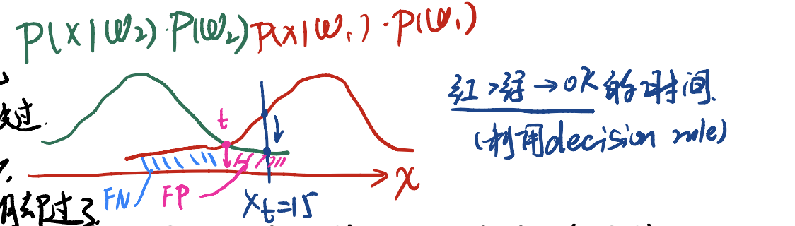
假设我们用上面的交叉点作为我们的decision rule。会发现：

• FP区域：上面已经用颜色标记出来。这部分人花了很多的时间，但没有通过DLCV课程。不过我们的rule认为他们一定能通过。这被称为False Positive。虽然rule认为他们通过了，但事实上没通过。
• FN区域：上面用蓝色标记出来。这部分人花了很少的时间，我们的rule认为他们不可能通过。但可能因为他们很聪明，从而通过了DLCV课程。这部分称为False Negative。

FP与FN都是我们利用判断的rule，却判断失误的部分。这部分可以用$FP + FN$来表示。

Additional Question: is cross point the best solution?

If we can fully see the whole PDF, yes!

Full Picture of 4 indicators

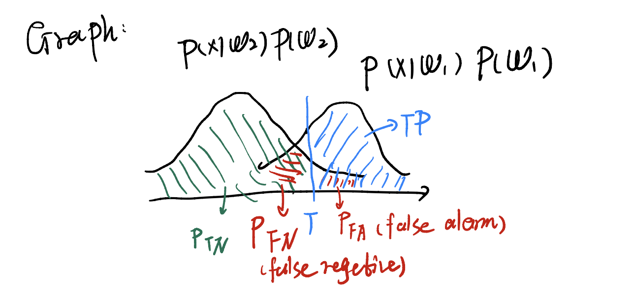
上图解释四个指标的关系。

• rejection(True Negative): 正确判断为$\omega_2$的部分。
• miss(false reject, FN): 错误判断的部分。这部分应该是通过的人，只是他们花的时间很少，不过却被rule给拒绝了。
• false alarm(FA, FP): 错误判断的部分。这部分人本身是没有通过的，但rule认为他们会通过，导致错误。
• true positive(TP): 正确判断为$\omega_1$的部分。

Receiver Operating Characteristics (ROC)

很多时候还涉及到比较两个model哪一个更好的问题，这就要请出ROC来帮忙判定。ROC曲线由两个坐标构成：$P_{FA}/FP$和$P_d / TP$​，即所谓的false alarm 和 detection 。

Deduction of RoC:

Case $1^\degree $: $T \rightarrow - \infty$

此时会有$P_{TP} = 1$（因为规则认为所有的都是通过的），且$P_{FA} = 1$ （另一条PDF都被囊括进去了），找到了点$(1, 1)$。

Case $2^\degree$: $T \rightarrow \infty$

此时会有$P_{TP} = 0$（因为规则认为所有的都是不通过的），且$P_{FA} = 0$ （另一条PDF都被囊括进去了），找到了点$(0, 0)$。

Case $3^\degree$: $T$在中间

此时必须要有$TP > FA$ 。因此应该在$45^\degree$线的上三角区域。

因此可以推导出下面的ROC曲线。

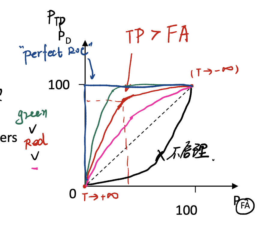
注意的是，曲线越向左上凸，model越好。

Clustering

If we use term like “clustering”, we mean no label we have to classified sorts of things. So, this is an unsupervised method.

Normally, we will give a set of $N$ unlabeled instances ${ x_1, …, x_N}$. And set the $#$ of clusters $K$.

Our goal is, to group the samples into $K$​ partitions.

Remark.

• For intra-cluster(aka within-cluster), we want it have high Similarity. (在一个cluster内，期望成员之间有很高的相似度)
• For inter-cluster(aka between-cluster), we want it have low Similarity. (在不同的cluster中，期望成员之间的相似度尽可能小)

So there comes a question: how to determine a proper Similarity measure?

Similarity

Similarity is a key component to perform data clustering. And it is inversely proportional to distance.

Here are some example distance metrics:

• Euclidean distance (L2 norm): $d(x, z) =

  x - z

  2 = \sqrt{\sum{i = 1}^D(x_i - z_i)^2}$

• Manhattan distance (L1 norm): $d(x, z) =

  x - z

  1 = \sum{i = 1}^D

  x_i - z_i

  $

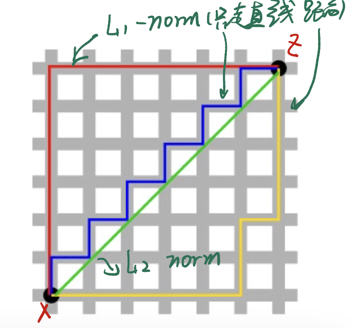
p-norm?

现在我们来定义所谓的p-norm。

\[L_p \text{-norm } = d(x, z) = ||x - z||_p, x,z \in \mathbb{R}^D\]

其中，

\[||x - z||_p = [\sum_{i = 1}^D |x_i - z_i|^p]^{1/p}\]

如果p变化，会有什么结果？

L0-norm

if $p \rightarrow 0$, we have…

当$p$趋近于$0$，我们知道只有非$0$数的0次方为1。因此，假如$p$趋近于$0$，可以让$

x_i - z_i

$中的非$0$项留下，而为$0$的项就从norm中除去了。因此，L0-norm的值就是$x_i \neq z_i$的个数。也就是 $#$​ of non-zero elements。

不过需要注意到，L0-norm不能微分！因此实际使用中如果我们希望筛选非0元素，常常用L1-norm来代替。

L$\infty$-norm

当$p \rightarrow \infty$，我们可以发现：

• 如果$

  x_i - z_i

  $的值很大，那这个值会被不断放大，$1/p$压不住这个值，会被留下来；

• 如果$

  x_i - z_i

  $的值很小，那这个值会被$1/p$压住，从而从norm中消失。

因此，$\infty$ norm可以用来筛选哪个attribute之间的距离最大，就留下哪一个来。

K-means clustering

这个算法非常经典，就不长篇大论介绍。

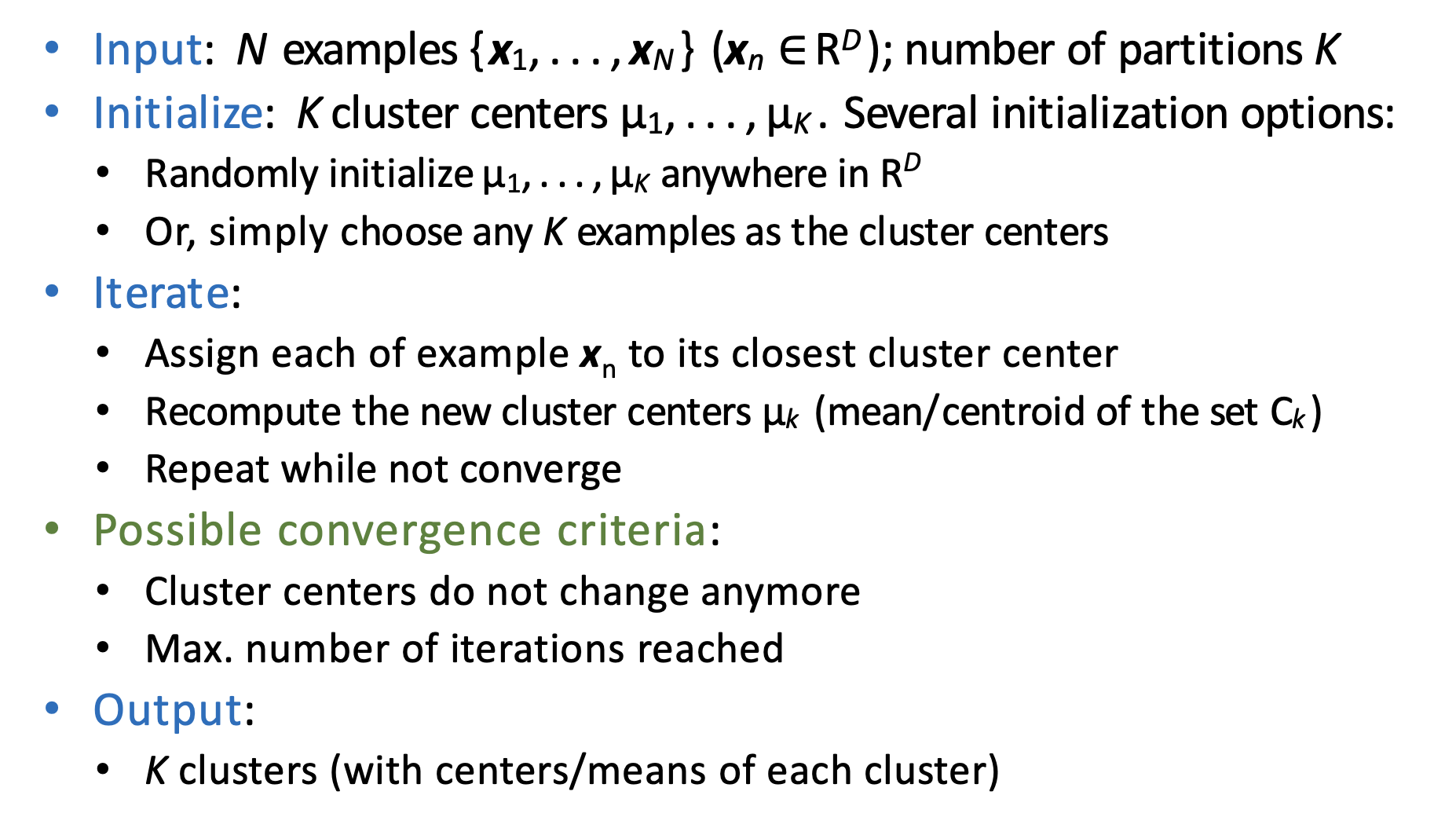
我们主要来介绍这个算法的优缺点。

Eazy to implement, but…

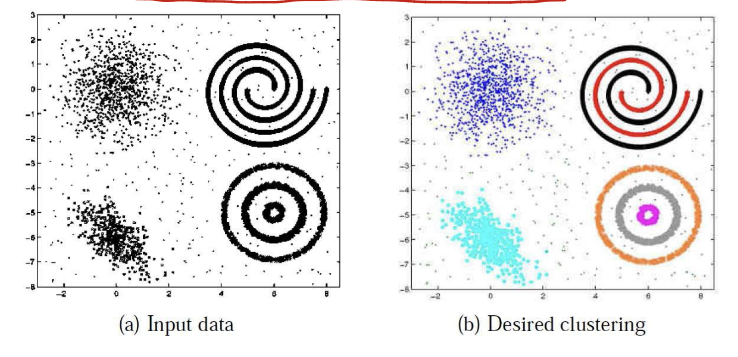
(1) 难以处理奇形怪状的数据

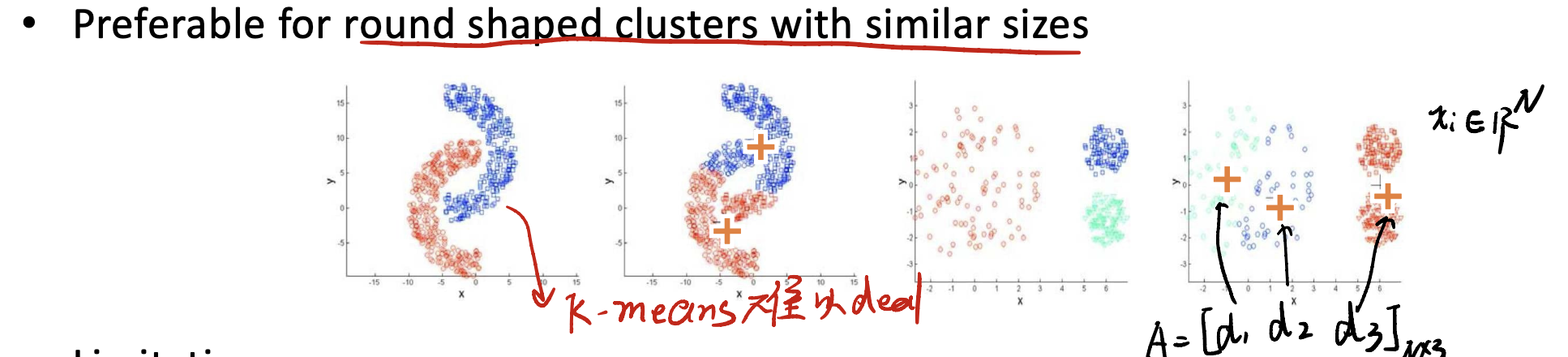
例如，像上面这种新月形数据，K-means非常难以处理。

(2) limitations

在K-means中，一个点只能属于某一个群，不能有“中间”状态。

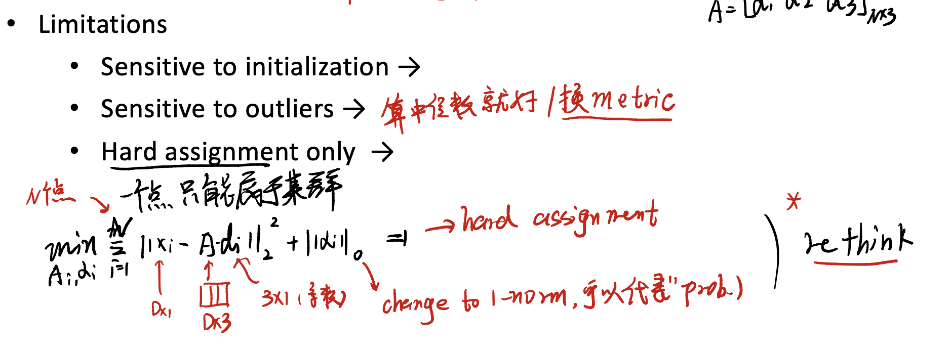
因此，我们还有其他的方法处理K-means遇到的问题。如：

• Expectation-maximization(EM) Algorithm
• Speed-up possible by herarchical clustering
• …

Training, Testing and Validation

Machine learning里，很重要的一部分就是所谓的训练、测试与验证。我们从Hyperparameter说起。

Hyperparameters in Machine Learning

很多情况下，我们需要提前决定好模型的超参数。如，K-means聚类的K是多少？CNN要用几乘几的convolution？科学起见，我们肯定不能靠猜测。

How to Determine Hyperparameter?

Use of validation data!

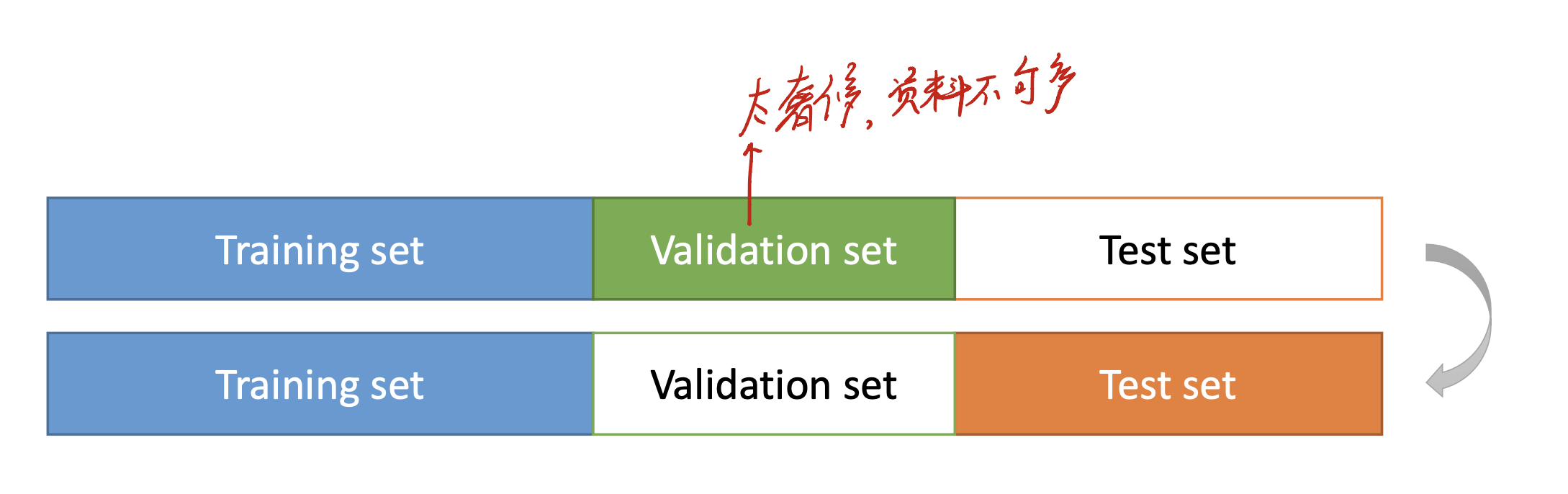
对于我们使用的data set来说，我们常常会把data set分为三个部分：training, validation, and test sets。

在train我们的model时，可以选择在validation set上表现得最好的hyperparameter，再去测试集上进行测试。

但……如果资料量不够多，我们的validation set分出来有点奢侈怎么办？

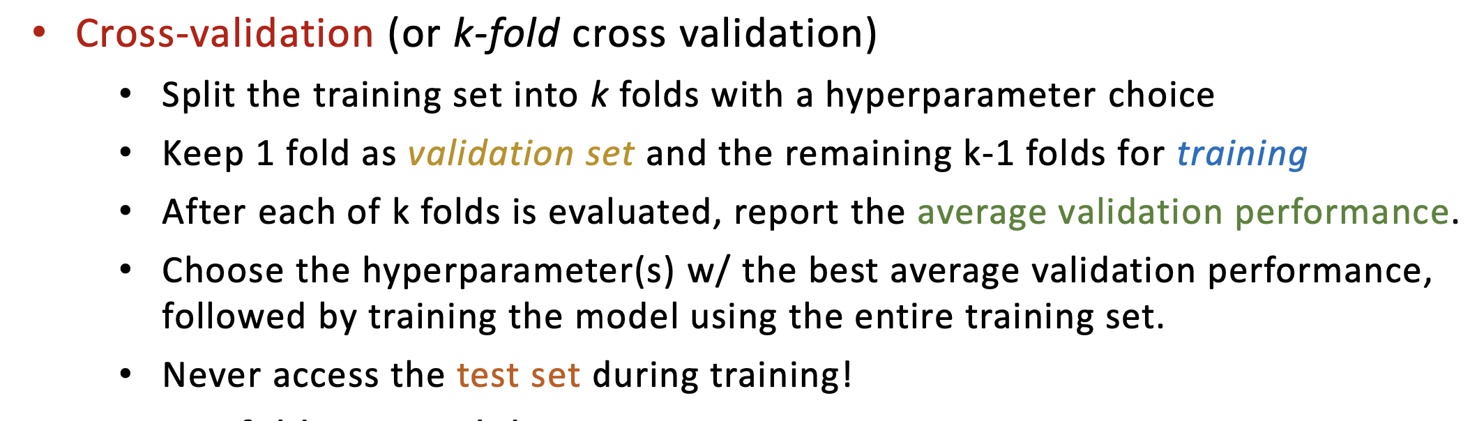
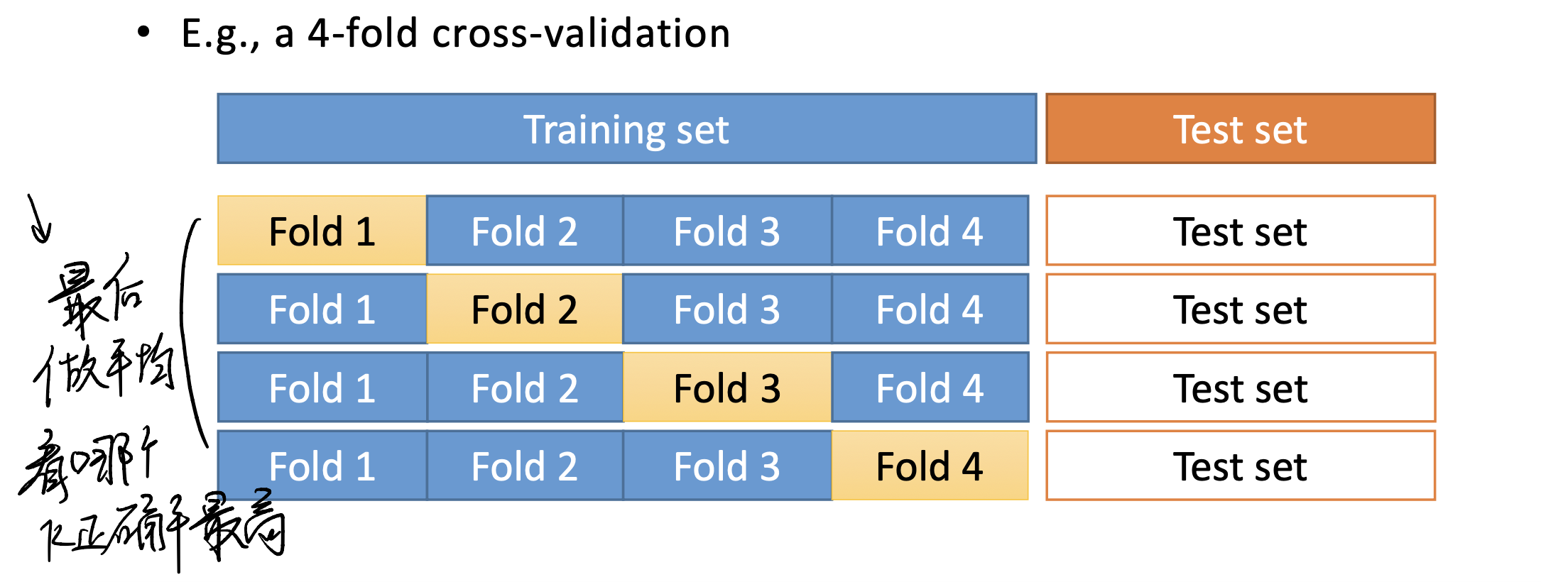
Cross validation helps! (or, k-fold validation)

这个时候要请出我们熟悉的k-ford cross validation来帮忙了。

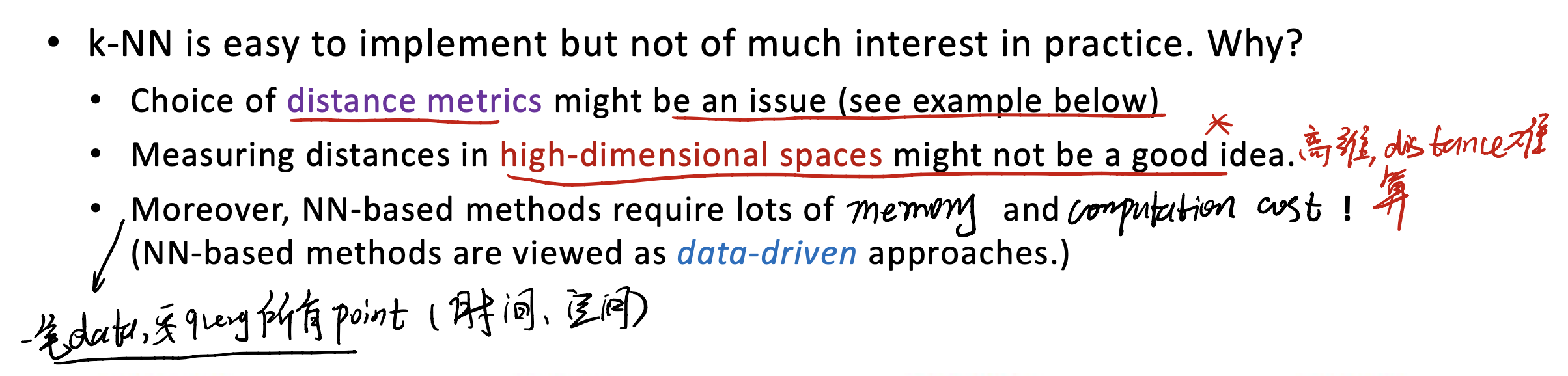
Minor Remarks on NN-based Methods

Linear Classification

Finally, let’s introduce the most famous question, which is, linear classification.

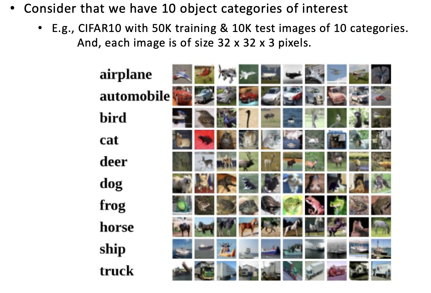
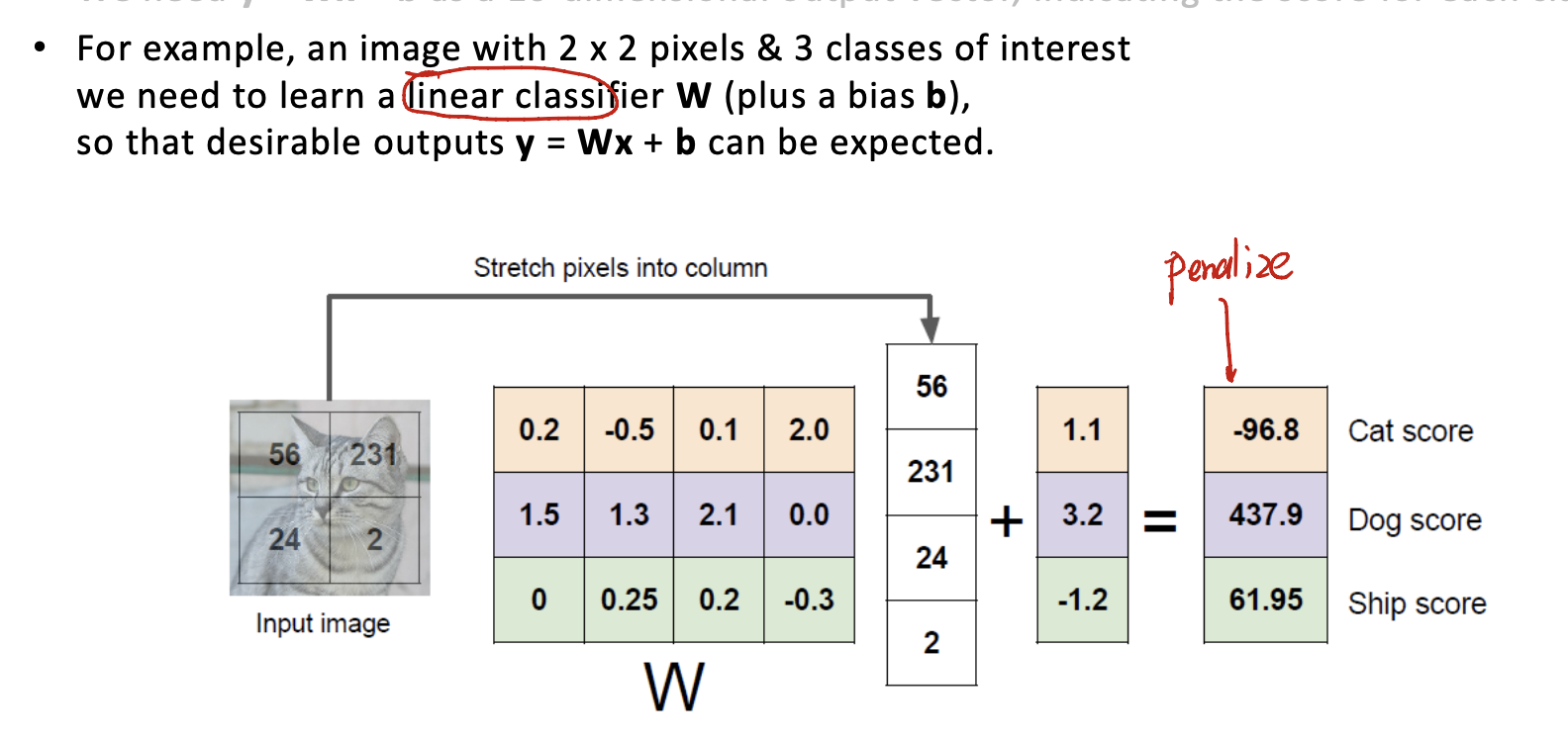
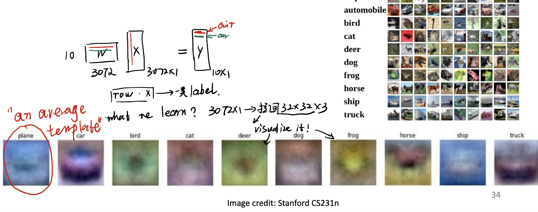
take input image as $x$, and the linear classifier as the parameter $w$. We need to find:

\[y = w^Tx + b\]

as a 10-dimensional output vector, indicating the score for each class.

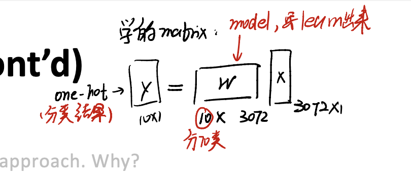
其实学的就是这个matrix而已。

Remarks

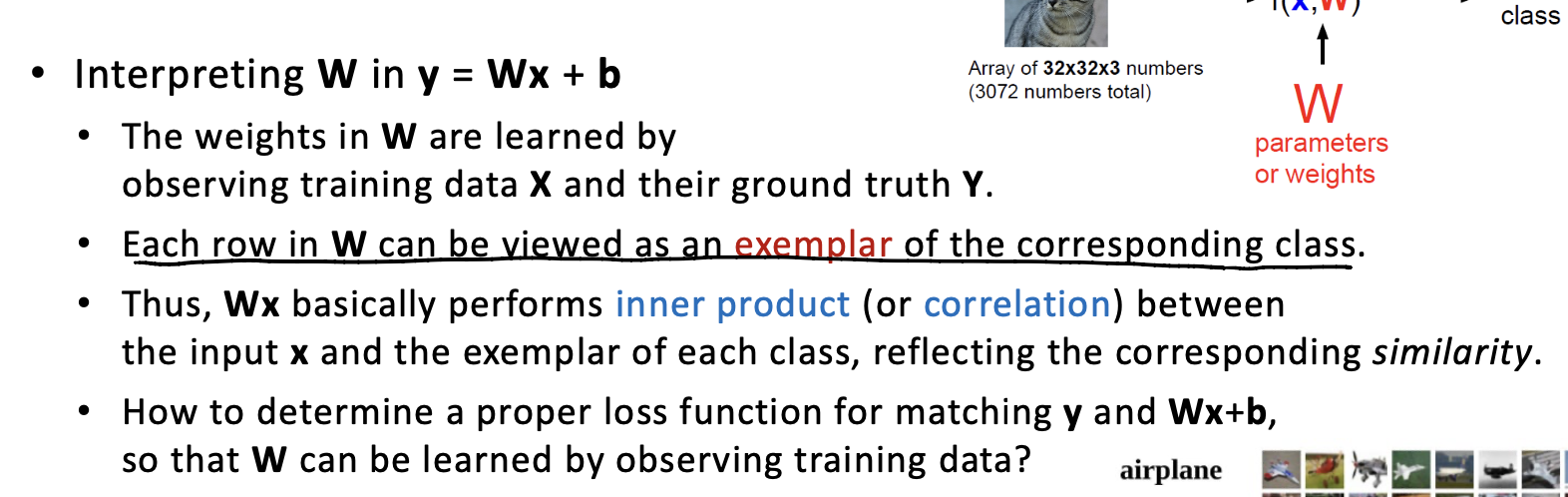
仔细考虑一下，在做矩阵乘法的时候，其实是把$w$中的某一行与整个input做内积。如果把w中的一行从flattern的状态中复原：会是一个$32 \times 32 \times 3$的图片。

那$w$到底学到了什么？或许是每一类图片的平均。$w$的每一行似乎是一种类别的平均长相，用这个类别的平均长相和待识别的picture做内积，从而得到一个相似度的结果。总共会有10种相似度，然后进行归类即可。

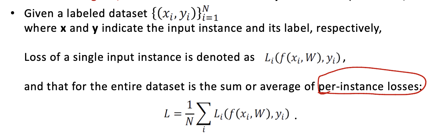
Loss Function

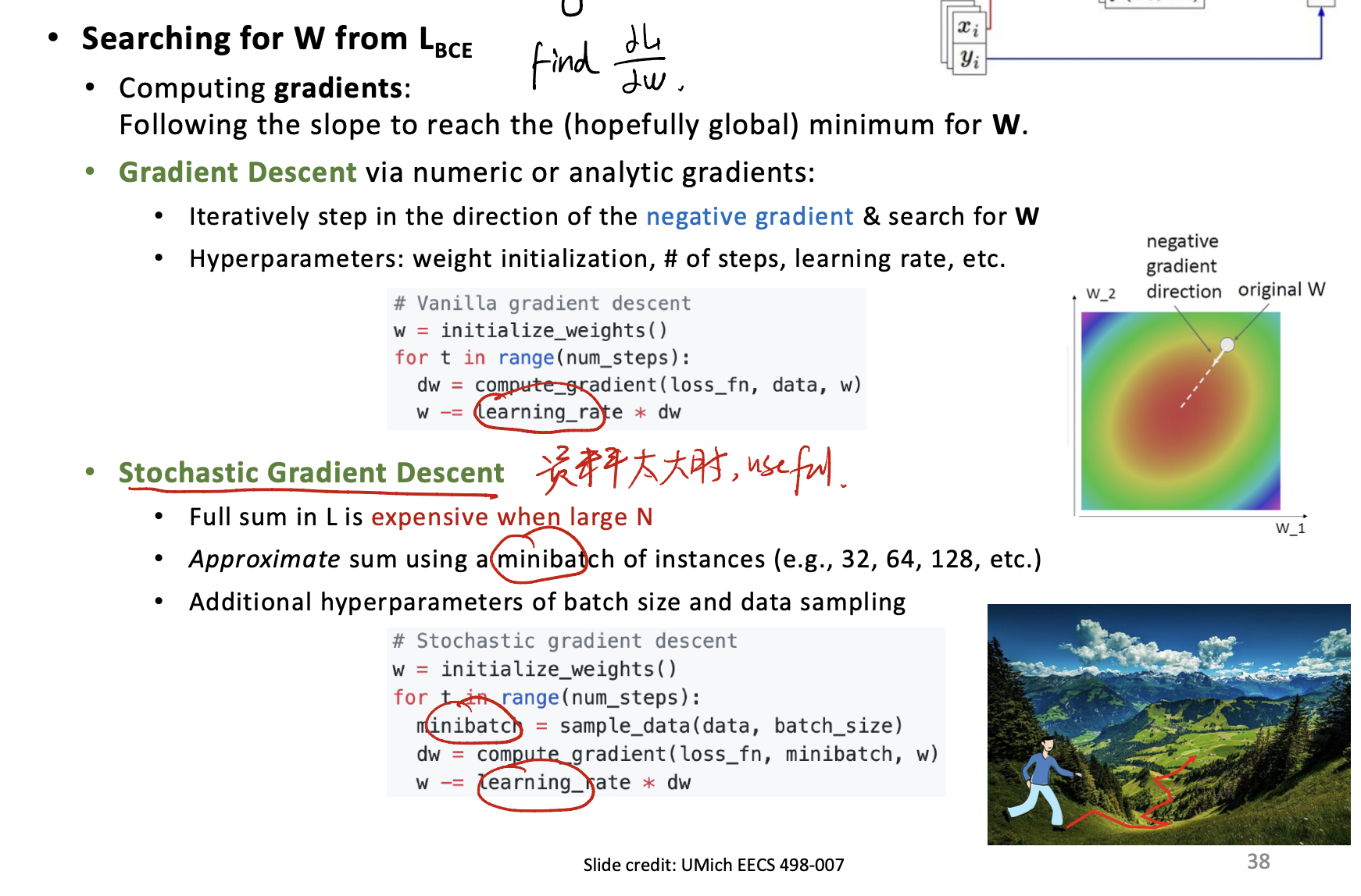
在learning的时候，需要来量化model的表现，这个时候就还是请出loss function来帮助我们判断了。Loss function负责告诉我们学到的参数$w$的好坏。The lower, the better。

Remark

在实作上，如果要计算全部的loss，是非常耗费运算资源和时间的。因此有所谓的mini batch的training方法，即一次喂给model一定个数的input，从而加快训练进程。

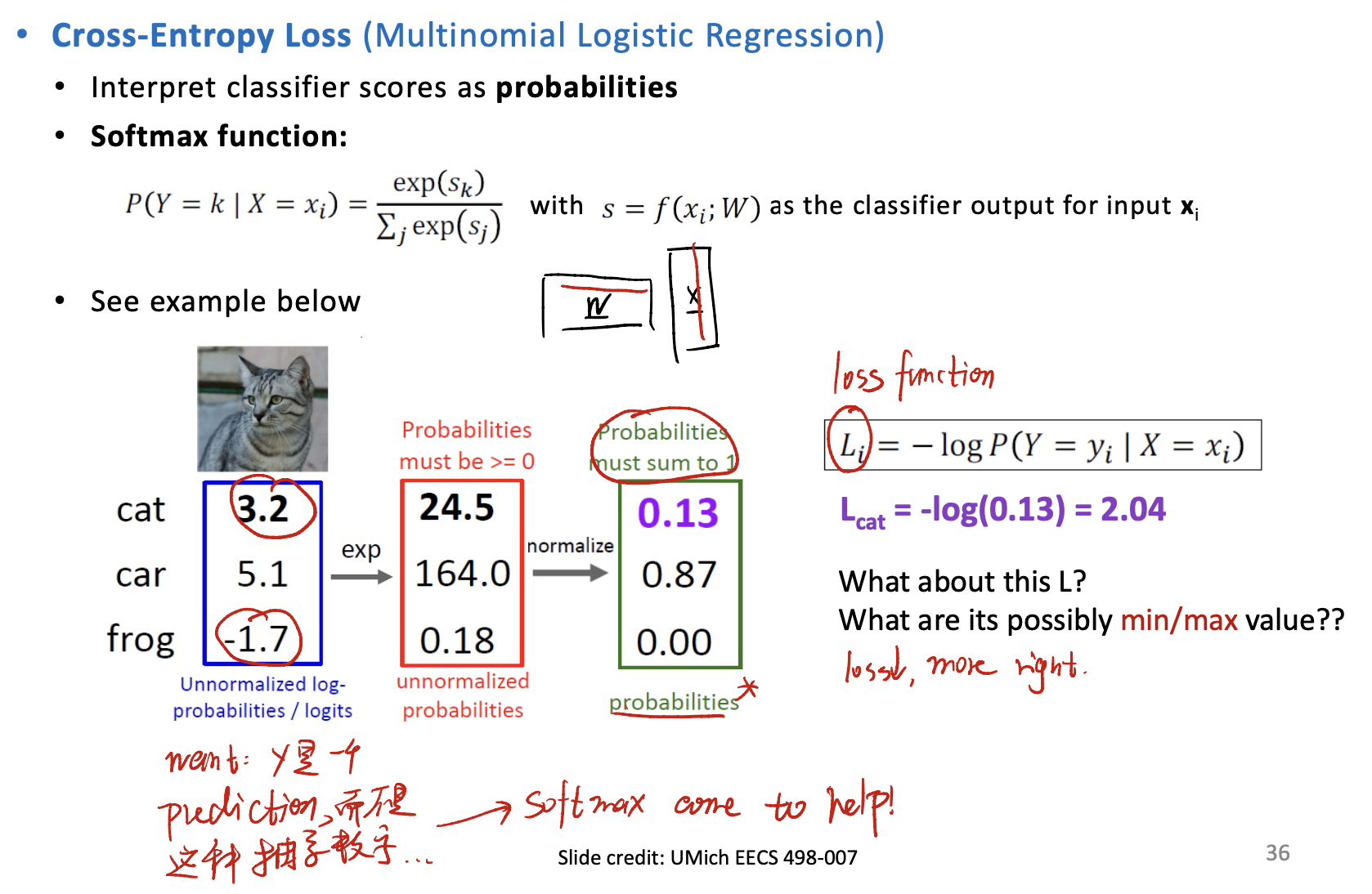
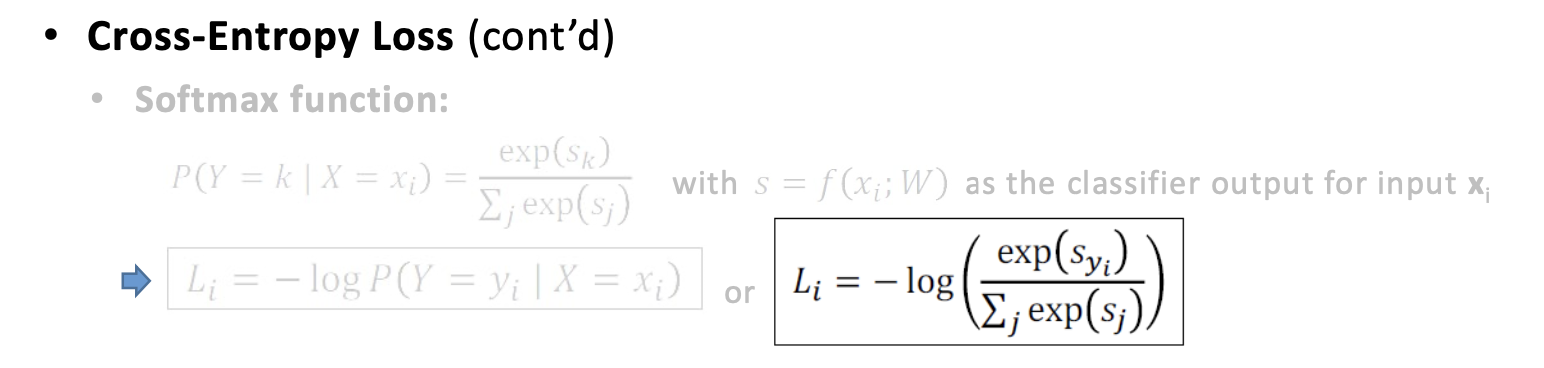
Cross-Entropy Loss and Softmax Function

Cross-Entropy Loss是非常常用的loss function。特别是在分类的loss计算上。

Cross-entropy is a measure from the field of information theory, building upon entropy and generally calculating the difference between two probability distributions. It is closely related to but is different from KL divergence that calculates the relative entropy between two probability distributions, whereas cross-entropy can be thought to calculate the total entropy between the distributions.

It is useful when training a classification problem with C classes. If provided, the optional argument weight should be a 1D Tensor assigning weight to each of the classes. This is particularly useful when you have an unbalanced training set.

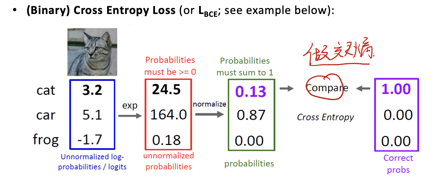
Binary Cross Entropy Loss ($L_{BCE}$)

注意所有的cross entropy的计算应该在做softmax之后，与one-hot vector进行比较。一个例子是：

Optimization::Gradient Descend

Reference

This notes comes from mostly National Taiwan Unviersity, COMME5052 Deep Learning and Computer Vision Course Slides. Thanks to Prof. Yu-Chiang Wang’s amazing teaching.