DA04 Dimension Reduction, Part IV
DA04 Dimension Reduction :: Part IV, Partial Least Squares Regression
In this note, we shall talk the last part of Dimension Reduction, which is Partial Least Squares Regression, (PLSR) .
We need to mind that PLSR is a kind of supervised method.
General Definition from Regression
首先从 regression 的定义说起。
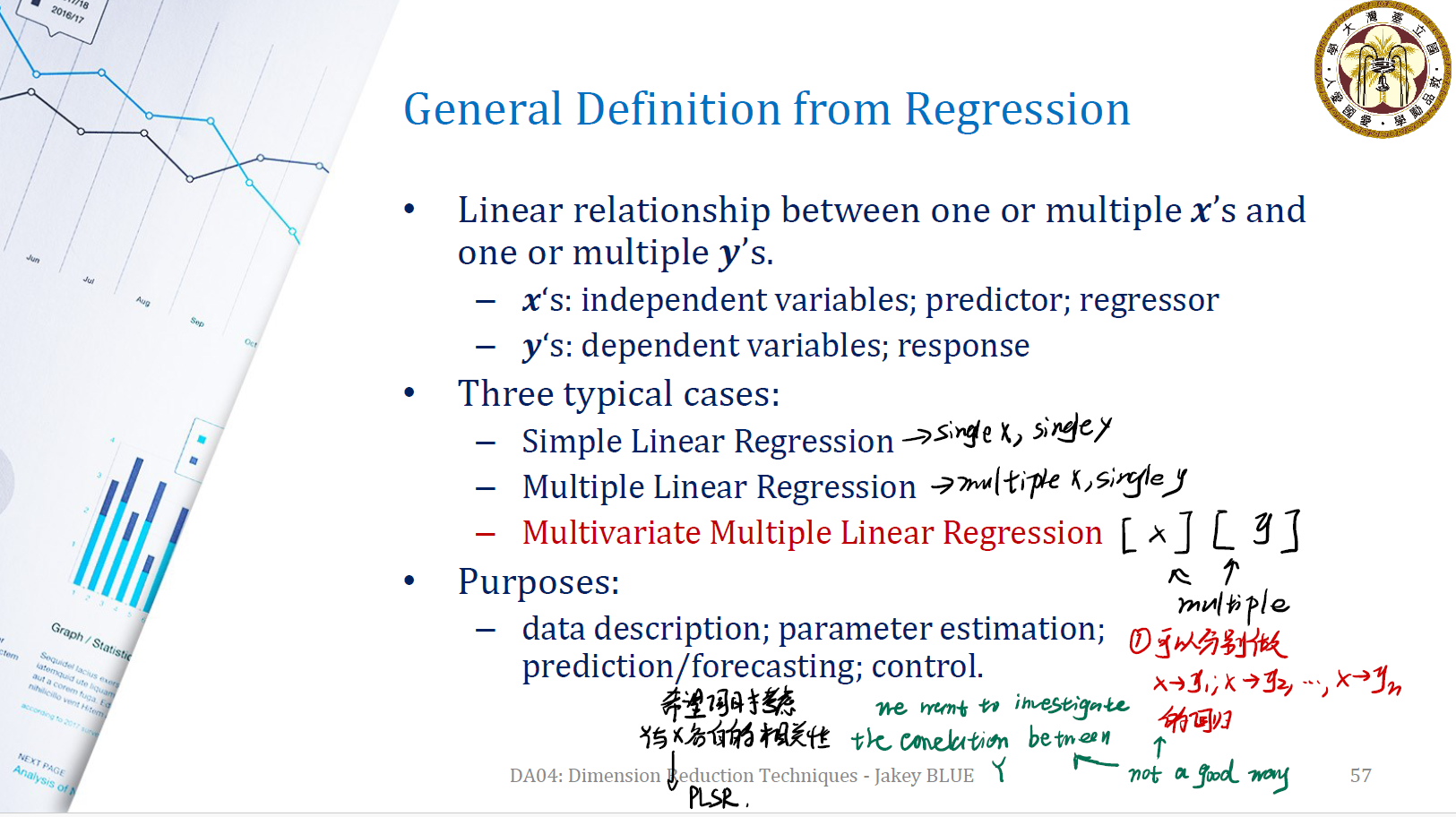
Definition 1. ( Linear Relationship ) 线性关系用来描述一个或多个 $x$ 与一个或多个 $y$ 之间的关系。其中:
- $x$: independent variables, predictor, regressor
- $y$: dependent variables, response
Definition 2. ( Type of Regression ) 具体而言,线性回归大概有三种: Simple linear regression, multiple linear regression, multivariate multiple linear regression 。
- Simple Linear Regression: single $x$ and single $y$. e.g. $y = b_0 + b_1x$
- Multiple Linear Regression: multiple $x$ and single $y$. e.g. $y = b_0 + b_1x_1 + … + b_p x_p$
- Multivariate Multiple Linear Regression: multiple $x$ and multiple $y$. e.g. $\mathbf{y} = \mathbf{X}\mathbf{\beta}$
那么,PLSR 又何谈 linear regression ?
Question PLSR Facing
Type-I Error inflation ?
考虑 Multivariate Multiple Linear Regression 的问题。我们有:
\[\begin{gathered} \begin{bmatrix} y_{11} & y_{12} & ... & y_{1q} \\ y_{21} & y_{22} & ... & y_{2q} \\ \vdots \\ y_{n1} & y_{n2} & ... & y_{nq} \end{bmatrix} \end{gathered}_{n \times q} = \begin{gathered} \begin{bmatrix} x_{11} & x_{12} & ... & x_{1p} \\ x_{21} & x_{22} & ... & x_{2p} \\ \vdots \\ x_{n1} & x_{n2} & ... & x_{np} \\ \end{bmatrix} \end{gathered}_{n \times p} \times \begin{gathered} \begin{bmatrix} \beta_{11} & \beta_{12} & ... & \beta_{1q} \\ \beta_{21} & \beta_{22} & ... & \beta_{2q} \\ \vdots \\ \beta_{p1} & \beta_{p2} & ... & \beta_{pq} \\ \end{bmatrix} \end{gathered}_{p \times q}\]我们要用变量 $x_1, …, x_p$ 这 $p$ 个 regressor 去估计 $y_1, … y_q$ 这 $q$ 个 response 。
一个很直觉的想法是分别对 $y_1, y_2, …, y_q$ 做 linear regression 。这样可以分别得出相应的回归方程式。
但显然不是一个好方法,与 ANOVA 相同,会增加类似于 Type-I Error 的概率。从而使得对 $y_1, …y_q$ 的估计不准确。
并且,分别做 regression 的方法没有考虑到 $y_1, …, y_n$ 之间的相关性,这也会造成一定的影响。
Challenges of Relationship Modeling
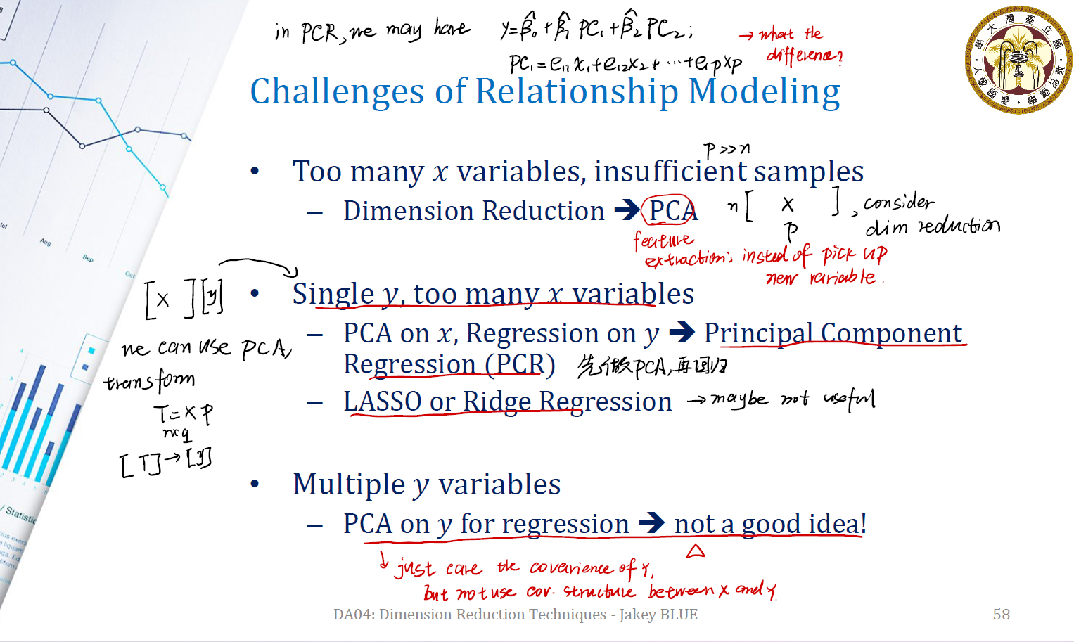
另一个问题是,如何在 insufficient samples (即 $p \gg n$ )的情况下进行 relationship modeling ?
$\longrightarrow$ 需要使用 Dimension Reduction 技术。例如 Principle Component Regression ( 主成分回归 )。
Step of Principle Component Regression:
- 先对 $x$ 做主成分分析,得到一系列主成分 $PC_1, PC_2, …, PC_p$ 。
- 随后,利用这些主成分对 $y$ 进行线性回归。回归式为 $y = b_0 + b_1 PC_1 + … + b_p PC_P$
当然,也可以使用 Lasso 或 Ridge Regression 来做。不过这不是一种推荐的做法。
同样,面对 multiple $y$ variables ,似乎也可以用 PCR 的方法来做。
Problem of PC Regression
PCR 如果这么好,那问题就到此结束了。实际上,PCR 有一个很致命的问题。
在主成分分析中,我们分析的是样本 $x$ 的 covariance matrix ,试图将样本投影到方差最大的方向上。这在 Dimension Reduction 是没有问题的。然而,在回归上,我们要做的是 $y$ 对 $x$ 的回归。那我们也应该考虑 $x$ 与 $y$ 之间的 covariance matrix 才对。PC Regression 并没有考虑这一点。
Information Loss in Dimension Reduction
在做 Dimension Reduction 的时候,到底丢失了什么信息?
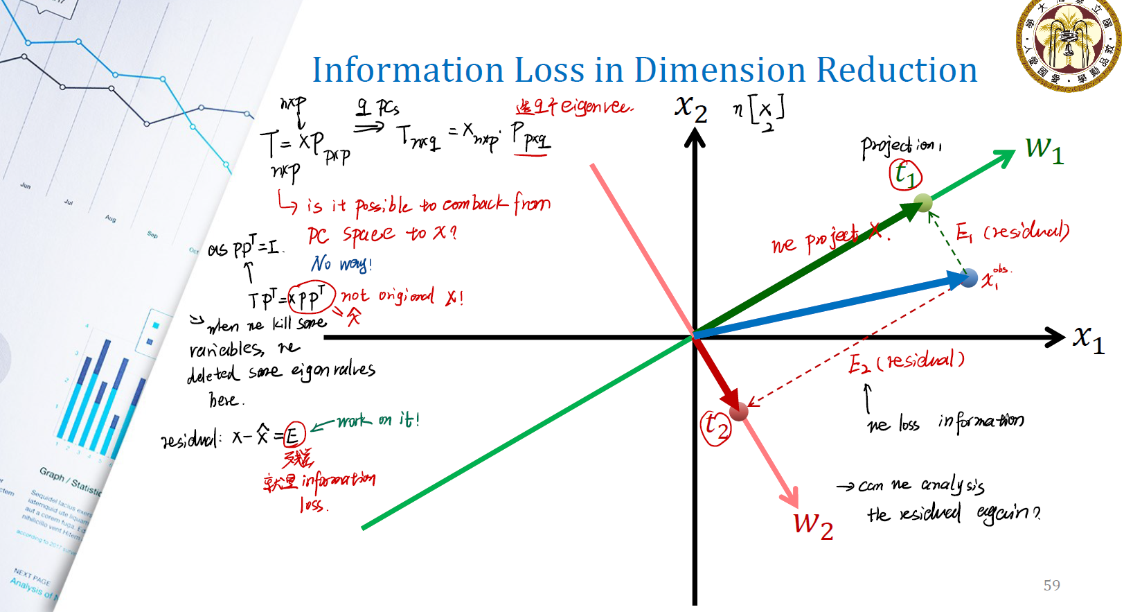
以 PCA 为例:
\[T_{n \times q} = X_{n \times p} \times P_{p \times q}\]如果没有 information loss ,则按照之前的分解得到的 $T$ 肯定能通过矩阵乘法的方式, transform 回原空间。由于矩阵 $P$ 是正交矩阵,故一定有 $P^TP = I$ 。因此:
\[T P^T = XPP^T = \hat{X}\]是否有 $PP^T = P^TP$ ?答案是 of course not !很显然,$PP^T$ 是一个 $p \times p$ 的矩阵,而 $P^TP$ 是一个 $q \times q$ 的矩阵。且 $P$ 不可逆,因此不可能有 $\hat{X} = X$ 。出现 information loss 。
因此有:
\[\text{residual} = X - \hat{X} = E\]图示上可以看成。在上图中,我们将观测值 $x_1^{obs}$ 利用主成分分析分解到方向 $w_1$ 与 $w_2$ 上,以期望用 $w_1, w_2$ 来替代观测值。因此产生的残差就是 $x_1^{obs} - t_1$ 与 $x_1^{obs} - t_2$ 。这就是我们丢失的信息。
Canonical Correlation Analysis (CCA)
下面我们先介绍所谓的典型相关分析。这也是一种 dimension reduction 方法,用来解释两个变量之间的关联关系。
与主成分分析不同。在主成分分析当中,我们主要分析数据集 $X$ 的 covariance matrix 。在 CCA 中,我们期望将 $X$ 和 $Y$ 一起分析,考虑 $X$ 和 $Y$ 的 covariance matrix 。
Our objective is, make largest correlation. Which means we need to maximize covariance matrix of (U, V). Where $U = Xw_x$ , $V = Yw_y$ .
\[\text{Objective: } \max cov[Xw_x, Yw_y] \Rightarrow \max w_x^T X^TYw_y\] \[\text{Subject to: } var[Xw_x] = 1, var[Yw_y] = 1\]我们期望 $Yw_y$ 和 $Xw_x$ 相比于 $Y$, $X$ 可以拥有更多的 information 。
几何意义是:
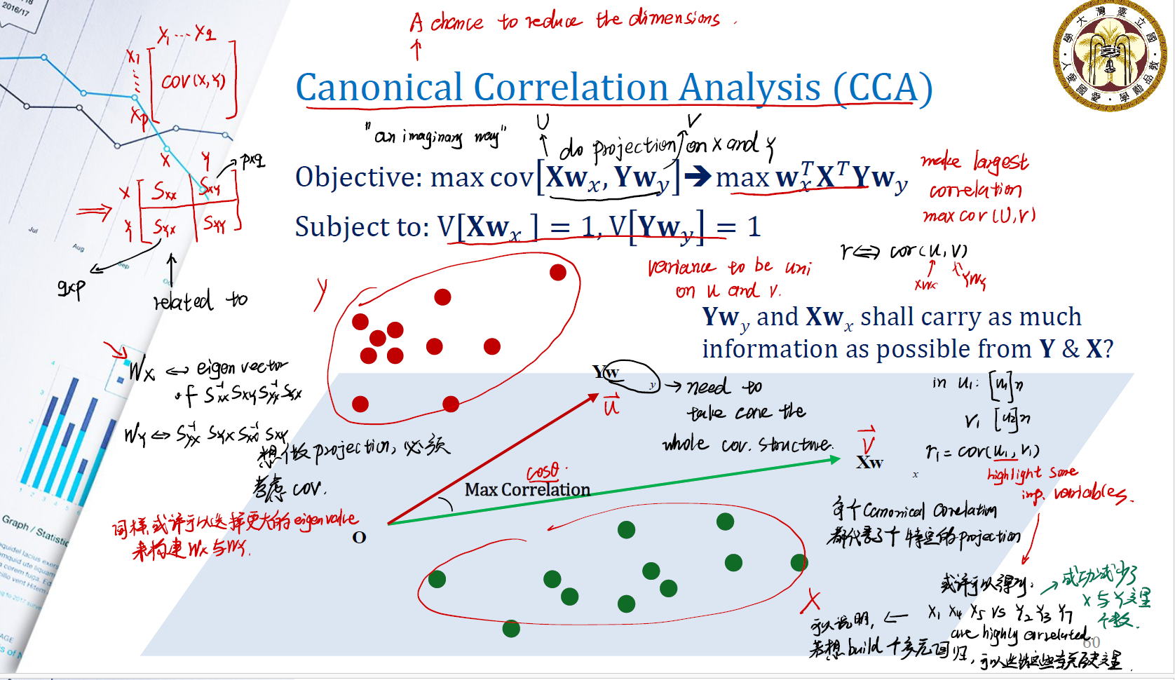
在 $X$ 的 column space 中,我们找到两个变量 $U, V$ 。期望它们之间的 corr 最大,在 column space 中,也就是 $\vec{v}, \vec{u}$ 。因此我们就是期望两个向量之间的夹角最大。
所以在 canonical correlation analysis 中:
- 每个 canonical correlation 都代表了一个特定的 projection 。
- 与 PCA 类似, $w_x$ 是矩阵 $S_{xx}^{-1}S_{xy}S_{yy}^{-1}S_{yx}$ 的特征向量; $w_y$ 是矩阵 $S_{xx}^{-1}S_{xy}S_{yy}^{-1}S_{yx}$ 的特征向量。
在分析后,可以找到 highly correlated 的变量,这样就能减少 $x$ 与 $y$ 的变量分析个数,成功做到 dimension reduction 。
Information Loss in Dimension Reduction
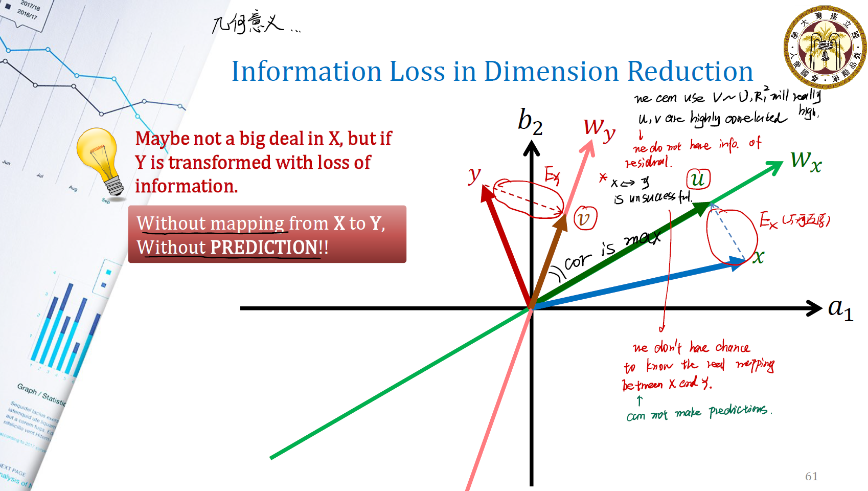
我们将原数据 $x, y$ 分别投影到令其方差最大的 $w_x, w_y$ 方向上,试图解释它们。但这样做总会舍弃掉投影的垂直部分,从而产生 information loss 。这样做的后果是,我们无法分析 residual 中的信息,也无法从 residual 中还原出有用的信息。此外,我们也无从得知,$x$ 是怎么转换生成对应的数据 $y$ 的,这意味着我们无法进行 prediction 。
Consider PCA, CCA, and Mapping Altogether
能不能将这三个部分结合起来,使得我们有机会将投影后的数据转换回投影前的数据呢?这也就是 PLSR 方法的重要设想。
In general, PLSR want to have chance to come back to original space to build the model.
简单来说,LDA将分类的标签作为降维的依据,而PLS将回归的数值作为降维的依据。
步骤为:
- Normalize $X$ and $Y$ . 要求
centered( 也就是均值为0 ) 与 divided by standard deviations ( 也就是标准差为 1 ) 。 - Find the linear combinations $p_1$ and $q_1$ , such that $u_1 = Xp_1$ and $v_1 = Yq_1$ . 这一步类似于 PCA ,也是找到 loadings 。
- Maximize $var[u_1]$ and $var[v_1]$. 在 CCA 中,我们需要 univariance 。而在现在,我们要最大化 variance ,以期为我们带来最多的 information 。
- Maximize $corr[u_1, v_1]$ 。
- 结合3,4可以发现,其实就是 Maximize $cov[u_1, v_1]$ 。
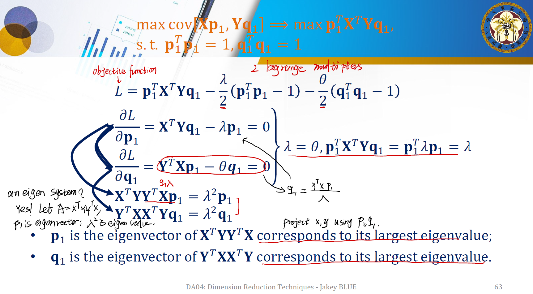
因此我们的最优化要求可以写成:
\[\text{Objective: } \max cov[Xp_1, Yq_1] \Rightarrow \max p_1^T X^TYq_1\]\(\text{Subject to: } p^T_1p_1 = 1, q^T_1q_1 = 1\) 接下来的分析求解与 CCA 的类似,同样是用 2 Lagrange multipliers ,我们得到:
Findings
我们做的其实是:
\[T_{n \times r} = X_{n \times p} P_{p \times r}\]很显然,没有 $P^TP = I$ 的条件,我们如果想要还原:
\[T_{n \times r} P^{-1}_{r \times p} = \hat{X}_{n \times p}\]这里的 $P^{-1}_{r \times p}$ 是矩阵 $P$ 的伪逆。在这里我们想用 regression 的方法来找到 pseudo inverse 。
$p_1$ 和 $q_1$ 试图在 PCA 和 CCA 两种方法之间找到一个平衡,其中的背景是:
- maximizing the variances of $Xp_1$ and $Yq_1$ .
- maximizing the correlation between $Xp_1$ and $Yq_1$ .
既然有了 $p_1$ 和 $q_1$ ,我们可以通过迭代的方法来求解 $u_1$ 与 $v_1$ :
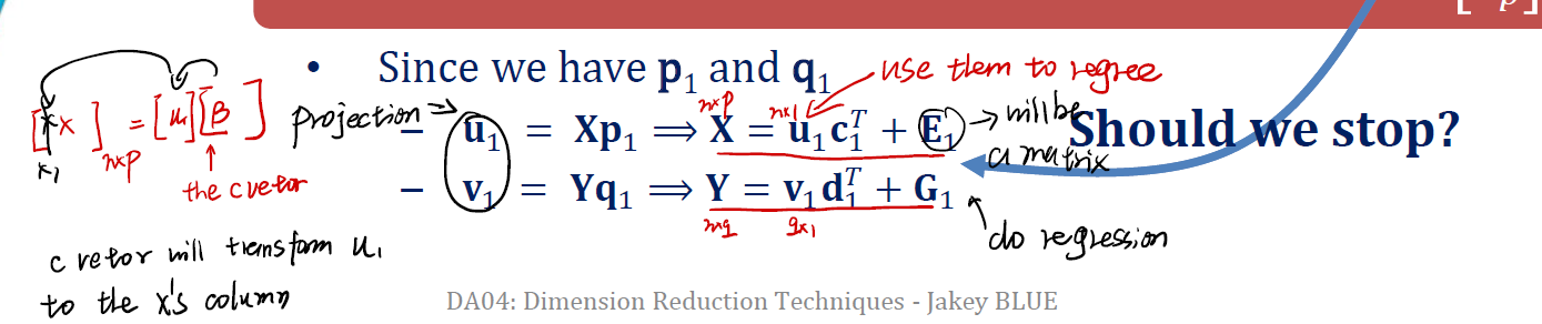
One Iteration of PLS Regression
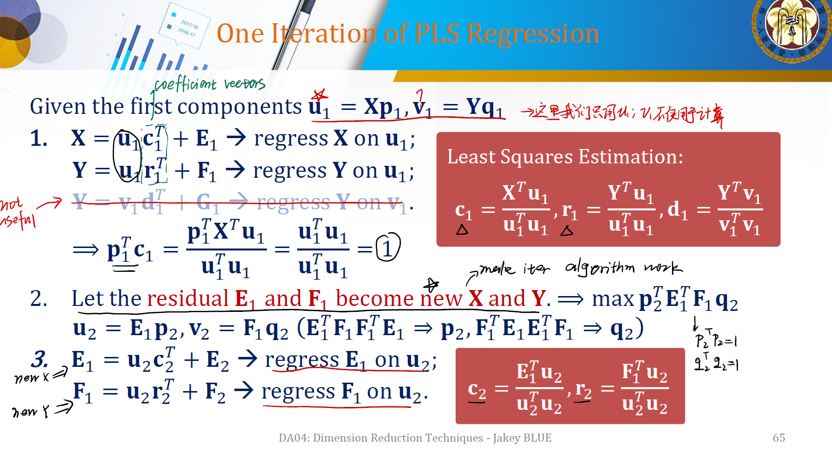
注意到我们的回归只是对 $u_1$ ,因为 $v_1$ 不方便计算…… 每一次迭代后,我们都让残差 $E_1$ 和 $F_1$ 当作新的 $X$ 和 $Y$ 。再进行相同的操作。
The Relationship Between Two Iterations
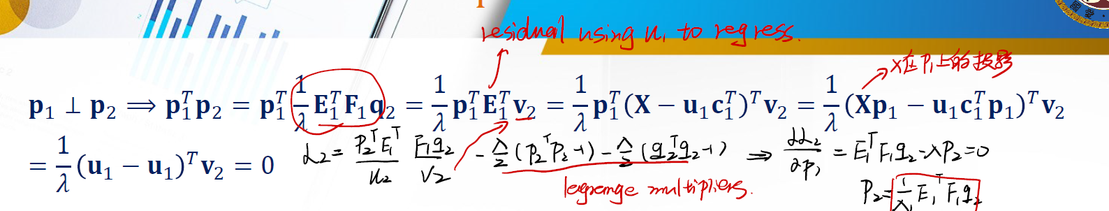
$p_1 \perp p_2$
这意味着 $p_1$ 与 $p_2$ 相互独立。让二者直接做内积可以证明:
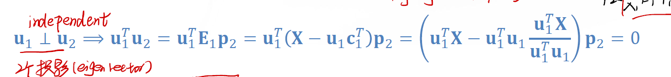
$u_1 \perp u_2$
同样意味着 $u_1$ 和 $u_2$ 之间相互独立。
$p_1 \perp c_2$
此外还有 $p_2 \perp c_1$ , $c_1 \perp c_2$ .
After Many Iterations…
在多轮次迭代后,会有:
\[X = u_1c_1^T + u_2c_2^T + ... + u_nc_n^T + E_n, \text{ all combinations of } u_nc_n\] \[Y = u_1r_1^T + u_2r_2^T + ... + u_nr_n^T + F_n, \text{ all combinations of } u_nr_n\]所以,
\[X = UC^T + E_n\] \[Y = UR^T + F_n = XPR^T + F_n = XB + F_n \text{, where } B = PR^T\]上面的 $B$ 就是我们的 loading matrix , $F_n$ 是最终的 residual 。并且, $\hat{Y} = X\hat{B} = X\hat{P} \hat{R}^T$ 。
- $Y$ is now actually the sum of many regression models.
- In the $i^{th}$ iteration, we collect $p_i, r_i$.
- To make prediction with new coming $x$, we can use $y^T = x^TB$
这样,我们似乎已经成功 extract 一些在 $X$ 与 $Y$ 之间的东西,利用最大化方差的方式,我们做了不一样的投影,在投影后,我们有最大化了相关系数。
Example: Wine Evaluation
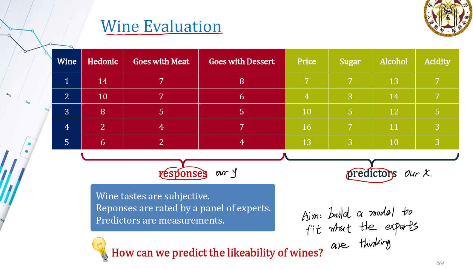
我们以 Wine Evaluation 来做一个例子。这个例子中有多个 predictors ,包括酒的价格、甜度、酒精度、酸度,来预测酒的三个特性。这是典型的 multiple X to multiple Y 的模型,可以用 PLSR 进行分析。
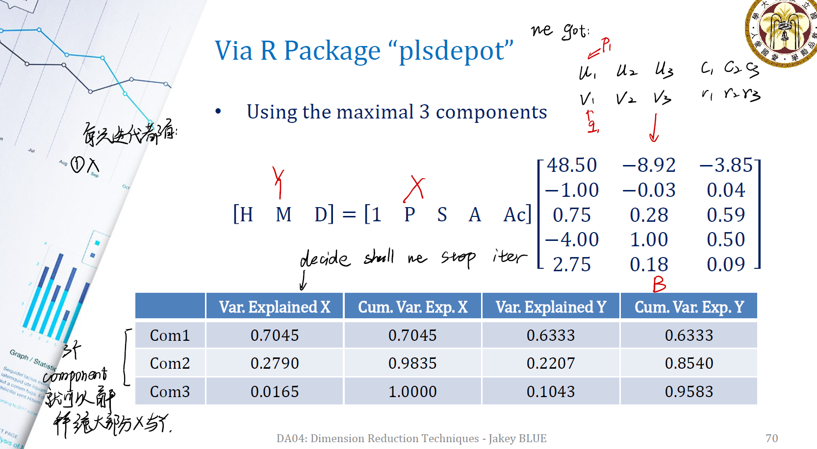
直接跑一个最简单的 PLSR 来进行分析,得到上面的 $Y = XB$ 的矩阵。
我们分解出了三个 component ,发现它们三个加起来在 $X$ 与 $Y$ 上都能有很接近于 1 的累计方差,这表明它成功地帮助我们解释了绝大部分的 $X$ 与 $Y$ ,实现了 Dimension Reduction 的目标。也可以利用这三个 com 来进行模型的构建与回归分析。
Reference
本文中的所有图片,Slides均来源于國立台灣大學工業工程學研究所藍俊宏副教授所開設的資料分析方法課程中之 DA04 Dimension Reduction.pdf。特此感謝藍俊宏老師在我學習歷程上的幫助!
其他参考: