DA04 Dimension Reduction, Part III
DA04 Dimension Reduction :: Part III, Factor Analysis
In this part, we will introduce another dimension reduction technology, Factor Analysys.
FA and PCA … What Different ?
Recall that PCA is to find the combination of the original variables, or, original dataset. We have:
\[T = X P\]where,
- $T$ is our Principle Components Matrix.
- $X$ is our original dataset.
- $P$ is the Loading Matrix, which is, to project original dataset $X$ to the new space. This is so-called Combination of original variables.
However, in Factor Analysis (FA) , we want to find latent (aka underlying) variables that can explain the original variables. It may like Hidden variables. ( 潜在的变量 ) We have:
\[X = FA\]where, $X$ is the known original dataset, or, original variables.
Generally speaking,
- In PCA, PC is unknown. We want to use original variables $X$ to
composePCs.- In FA, we have $X$ known original variables. And we decide to de-compose $X$.
Decomposition ?
Previously, we have already known that we want to decompose original $X$ to $FA$ . Let’s borrow the concept of SVD.
\[X = UDV^T\]where,
- $X$ is a $n \times p$ matrix, this is the original variable matrix.
- $U$ is a $n \times n$ matrix, and it is orthogonal, $U^TU = I$.
- $D$ is a $n \times p$ diagonal matrix.
- $V$ is a $p \times p$ matrix.
What we do to connect this decomposition with $X = FA$ ?
Let $F = \sqrt{N} UD$, and let $A = V^T / \sqrt{N}$ .
For decomposition of $F$ :
- we use $\sqrt{N}$ to rescale $F$.
- $N$ maybe a matrix, to rescale each column of $F$.
- $F$ is composed of uncorrelated variables with unit variances. ( $\sigma^2 = 1$ )
So, we have:
\(X_{n \times p} = F_{n \times p} A_{p \times p}\) We also need to mind that $F$ is not unique. Given any orthogonal $p \times p$ matrix $R$, we can always let $FA$ become $FR^TRA$, then combine $FR^T$ to new $F^\ast$, and $RA$ to new $A^\ast$.
How about unit variance? $cov(F^*) = R^T cov(F) R = I$ , ( why?1 ) still have unit variance.
However …
- We know that $F$ is a $n \times p$ matrix, this means $F$ has $p$ factors. However in our initial case, $X$ also has $p$ variables! ( Recall that our target is we want to find latent factors and reduce the number of factors ) How to use $p$ factors in $F$ to explain $p$ variables in $X$ ?
- And, how about explanation?
We shall deal with this issues later.
Reducing $p$ to $q$ ( $q \lt p$ )
Our target is reducing. we want to use $q$ factors. So,
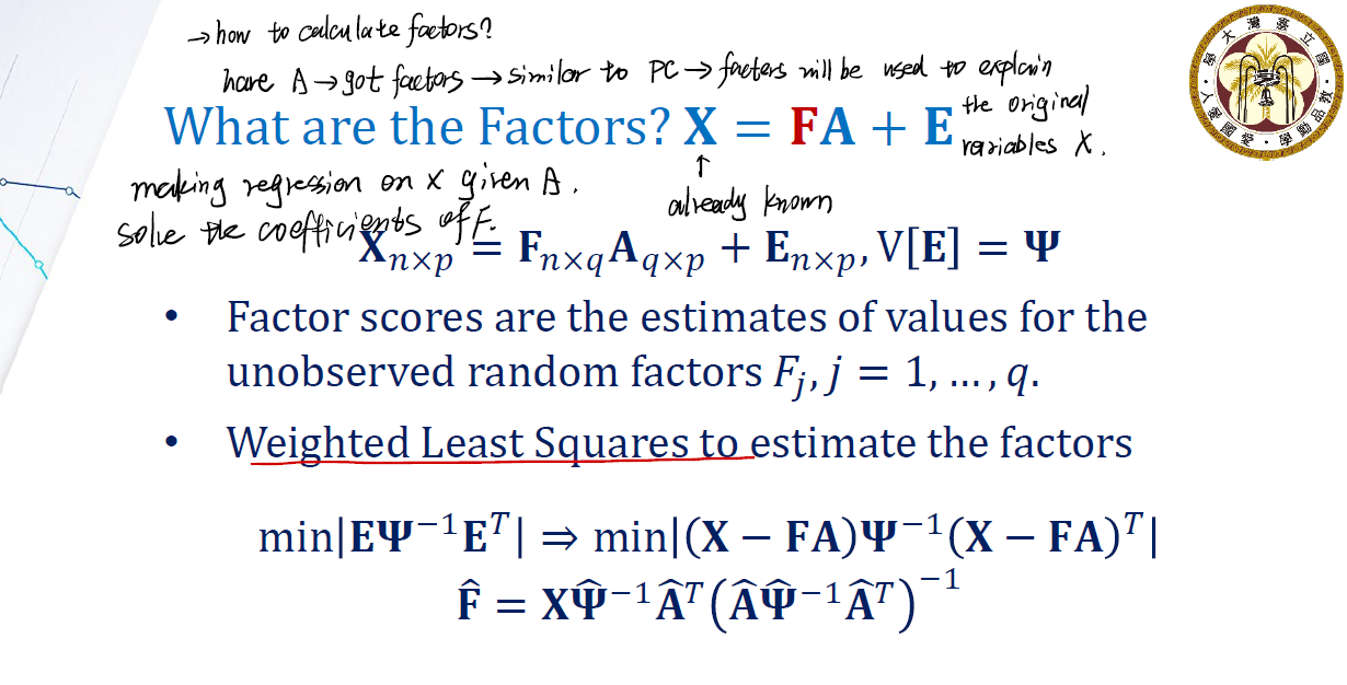
\[X_{n \times p} = F_{n \times q} A_{q \times p} + E_{n \times p}\]Open it,
\[\begin{gathered} \begin{bmatrix} x_1 & ... & x_p \end{bmatrix} \end{gathered} = \begin{gathered} \begin{bmatrix} f_1 & ... & f_q \end{bmatrix} \end{gathered} \times \begin{gathered} \begin{bmatrix} a_1 & ... & a_p \end{bmatrix} \end{gathered} + \begin{gathered} \begin{bmatrix} \epsilon_1 & ... & \epsilon_p \end{bmatrix} \end{gathered}\]- $[f_1, …, f_q ]$ is $q$ factors. The covariance of the matrix $F$ is $I$ (Univariance).
- $[a_1, …, a_p]$ is $p$ loadings.
- $[\epsilon_1, …, \epsilon_p]$ is $p$ residuals. Dimension of matrix $E$ is same as the dimension of matrix $X$.
As we try to use $q \ll p $ factors, we surely get residual.
And, for more opening step,
\[\begin{gathered} \begin{bmatrix} x_1 & ... & x_p \end{bmatrix} \end{gathered}_{n \times p} = \begin{gathered} \begin{bmatrix} f_1 & ... & f_q \end{bmatrix} \end{gathered}_{n \times q} \times \begin{gathered} \begin{bmatrix} a_{11} & ... & a_{qp} \\ \vdots & \ddots & \vdots \\ a_{q1} & \dots & a_{qp} \end{bmatrix} \end{gathered} + \begin{gathered} \begin{bmatrix} \epsilon_1 & ... & \epsilon_p \end{bmatrix} \end{gathered}_{n \times p}\]We are interested in the middle matrix $A$, which is our loadings. We can reduce $p$ to $q$ !
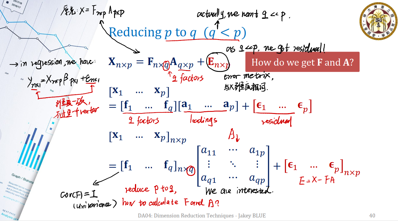
So how to get $F$ and $A$ ?
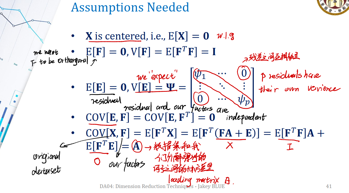
Assumptions in Factor Analysis
We also need assumptions for factor analysis.
- $X$ is centered. i.e., $E[X] = 0$.
- For Factor Matrix $F$, we want:
- $E[F] = 0$
- $var[F] = E[F^TF] = I$
- $F$ is orthogonal
- For residual matrix $E$, we want:
- $E[E] = 0$
- $var[E]$ is a diagonal matrix, with $\psi_i$ on the diagonal, and other place are all 0. ( 这意味着 residual 之间是互相独立的,并且 $p$ 个 residual 都有它自己的方差 $\psi_i$ )
- $cov(E,F) = cov(E, F^T) = 0$ ( residual and our factors are independent )
- $cov(X, F) = E[F^TX] = E[F^T(FA + E)] = E[F^TF]A + E[F^TE] = A$ ( 数据集 $X$ 和我们分解得到的 factor 之间的协方差是 loading matrix $A$ )
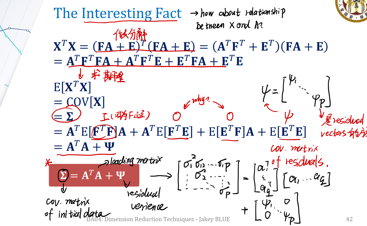
Interesting Facts
After our assumptions, we have some interesting facts.
Mind that our decomposition is $X = FA + E$. We surely wang to ask, how about relationship between $X$ and $A$ ?
$\longrightarrow$ For $X^TX$,
\[\begin{eqnarray} X^TX &=& (FA + E)^T (FA + E) \nonumber \\ ~ &=& (A^TF^T + E^T)(FA + E) \nonumber \\ ~ &=& (A^TF^TFA + A^TF^TE + E^TFA + E^TE) \nonumber \end{eqnarray}\]Calculate expectation of $X^TX$ on $F$,
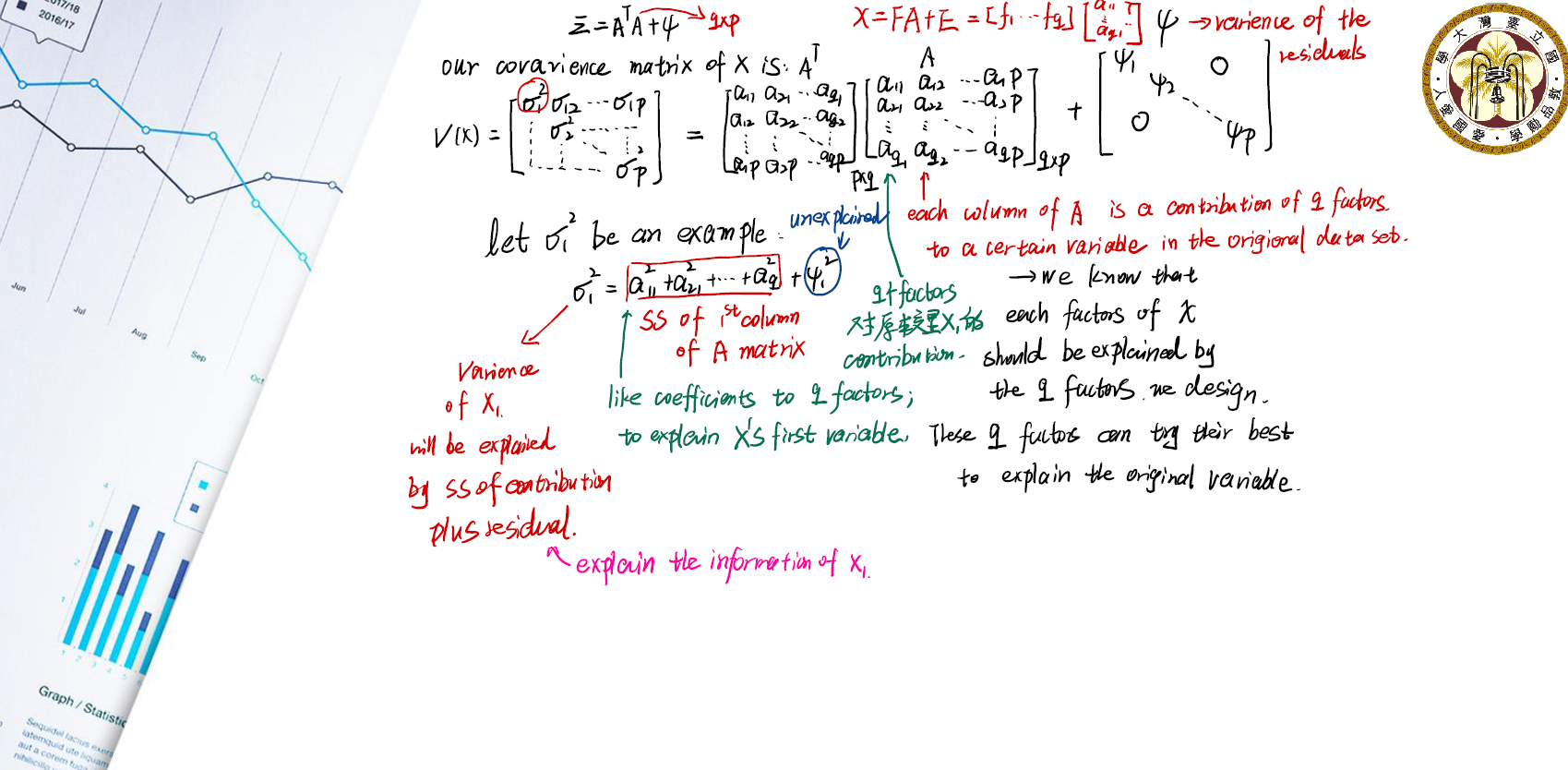
\[\begin{eqnarray} E[X^TX] &=& cov(X) \nonumber \\ ~ &=& A^TE[F^TF]A + A^TE[F^TE] + E[E^TF] + E[E^TE] \nonumber \\ ~ &=& A^TA + 0 + 0 + \psi \nonumber \\ ~ &=& A^TA + \psi \nonumber \end{eqnarray}\]也就是说,初始数据 $X$ 的 covariance matrix $\Sigma$ 为:
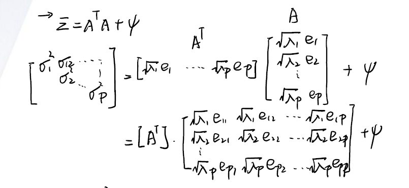
\[\Sigma = A^TA +\psi\]$A$ is loading matrix, and $\psi$ is residual variance.
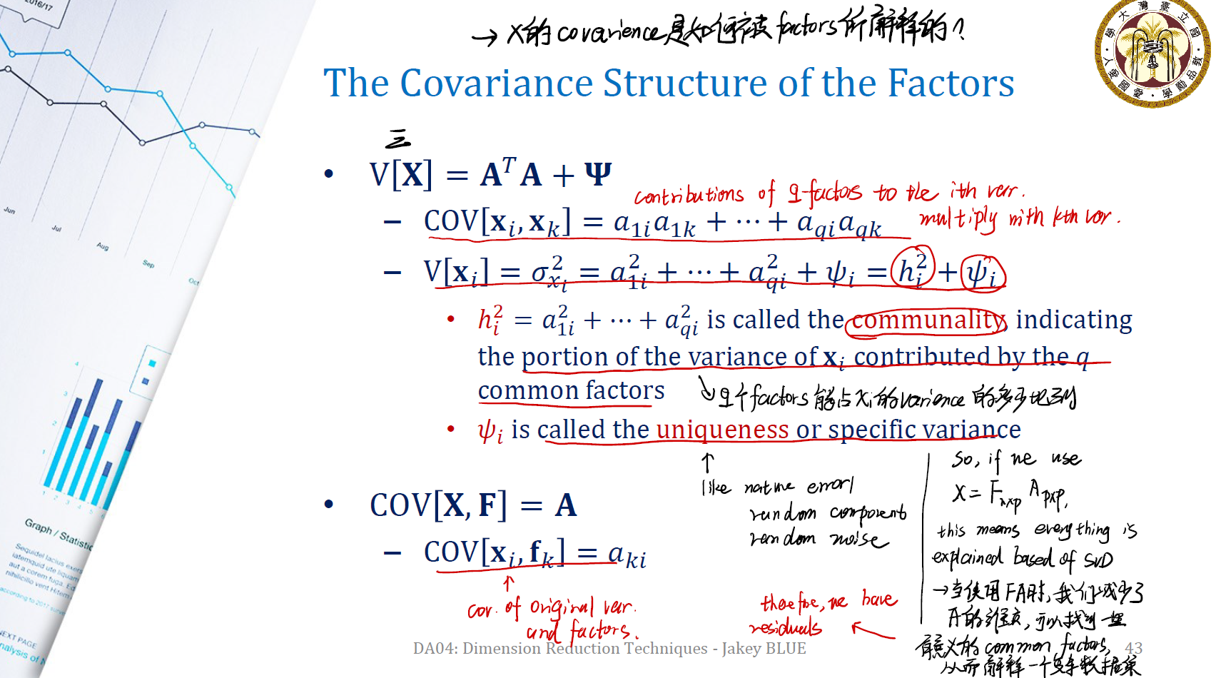
Covariance Structure of the Factors
我们还想知道数据的 covariance 是如何被我们分解得到的 factors 所解释的。因此,我们要分析数据矩阵的 covariance matrix。
考虑初始数据矩阵 $X$ 的 covariance matrix。在上一部分我们知道了 $X$ 的协方差矩阵 $\Sigma$ 的表达式:
\[cov(X) = \Sigma = A^TA + \psi\]对于第 $i$ 个 variable $x_i$ 与第 $k$ 个 variable $x_k$ ,我们有协方差:
\[cov(x_i, x_k) = \sigma_{ik} = \mathbf{a}_i^T \mathbf{a_k} = a_{1i}a_{1k} + \dots + a_{qi}a_{qk}\]同样,对于第 $i$ 个 variable $x_i$ ,我们有方差:
\[V[x_i] = \sigma^2_{x_i} = a^2_{1_i} + \dots + a^2_{q_i} + \psi_i = h_i^2 + \psi_i\]$h_i$ 被称为
communality,它表示我们选出的 $q$ 个 factors 能解释 $x_i$ 多少比例的 variance 。$\psi_i$ 被称为
uniqueness或specific variance。这类似于一个 nature error / random noise 。
在之前的推导 ( Assumptions ) 中,我们已经知道了 $cov(X, F) = A$ 。这也意味着 $cov(x_i, f_k) = a_{ki}$ ,即,原本的 variable 和 factor 之间的协方差是 loading matrix 中的某个对应元素。
Why residual ?
如果我们直接用一个分解 $X = F_{n \times p} A_{p \times p}$ ,矩阵 $A$ 的 column 的维度与 $X$ 的相同,这是一种所谓的“everything is explained” 。
而在 Factor Analysis 中,我们既然想要做到 dimension reduction 的目标,就要减少 $A$ 的 column 维度,从而找到有意义的 common factors ,来解释一个复杂的数据集。这样我们自然会因为维度减少而得到残差。
$A$ is not unique
Our decomposition is,
\[X = FA + E\]Given an orthogonal matrix $T_{q \times q}$ , so that $T^TT = I$. We have,
\[X = FA + E = FT^TTA + E = (FT^T)(TA) + E = F^\ast A^\ast + E\]How about our assumptions? In previous part, we want for Factor Matrix $F$, $E[F] = 0$, $var[F] = E[F^TF] = I$ and $F$ is orthogonal.
\[E[F^\ast] = E[FT^T] = E[F] T^T = \mathbf{0} T^T = 0\]for orthogonal,
\[(F^\ast)^T = (FT^T)^T \\ (F^\ast)^T F^\ast = (FT^T)^T FT^T = TF^TFT^T = TIT^T = I\]and for variation,
\[var[F^\ast] = var[FT^T] = E[(FT^T)^T(FT^T)] = E[TF^TFT^T] = TE[F^TF]T^T = TE[I]T^T = I\]new factor is also univariance.
显然,三个条件都满足。这样的变换是成立的。
同样,对于 covariance matrix of $X$, we also have,
\[\Sigma = (A^\ast)^T(A^\ast) + \psi\]因此我们有:
- Loading Matrix $A$ 由矩阵 $T$ 来决定。
- 前面在covariance structure 提到的 communalities, 矩阵 $A^TA$ 的对角线元素不随着 $T$ 的变化而变化。
Estimate $A$ by Principal Component
In this part we want to answer the question, How to calculate $A$ ?
我们想利用 主成分分析 的方法来解 loading matrix 。
首先对原数据集 $X$ 的协方差矩阵进行特征值分解:
\[\Sigma_{p \times p} = Q \Lambda Q^T = Q \sqrt{\Lambda} \sqrt{\Lambda} Q^T = A^T_{p \times p} A_{p \times p} + \mathbf{0}\]这是所谓的 fully decompose 。
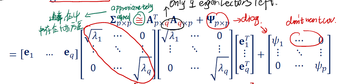
不过我们之前提过,我们期望将 variable 的数量从 $p$ 减少到 $q$ 。因此一个直观的想法是,我们忽视掉那些小的特征值,留下 $q$ 个显著的特征值。
As we always want to use $q$ factors, we have to sacrifice some eigenvalues!
所以这里我们的 covariance matrix 要修改成:
\[\Sigma_{p \times p} \simeq A^T{p \times q} A_{q \times p} + \psi_{p \times p}\]这里出现 $\psi$ 是因为我们缩减了规模,所以出现了 residual 。
打开的话,我们可以得到:
从而,得到 loading matrix 的关于原数据集 $X$ 的协方差矩阵 $\Sigma$ 的特征值和特征向量估计式:
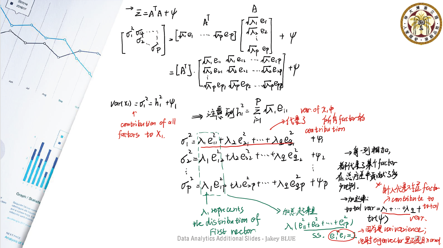
\[A^T_{p \times q} = \begin{gathered} \begin{bmatrix} \sqrt{\lambda_1} \mathbf{e}_1 & ... & \sqrt{\lambda_q} \mathbf{e}_q \end{bmatrix} \end{gathered}\]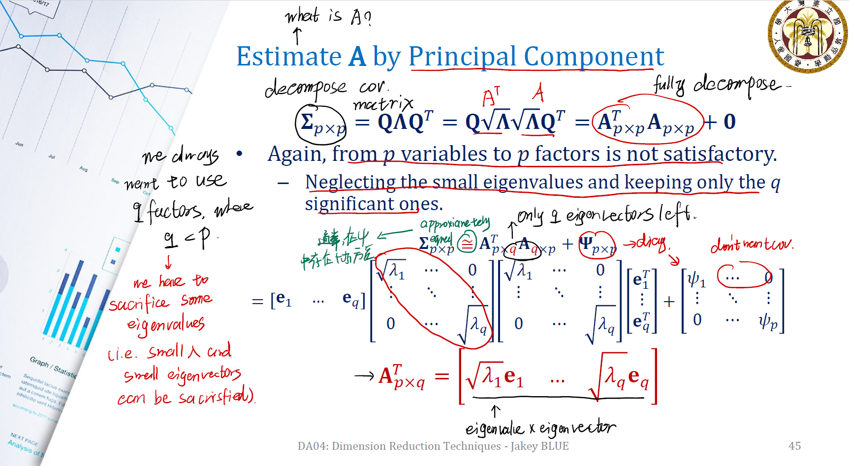
现在来分析 $\Sigma$ :
打开矩阵,前面已经定义了 communality :
\[var[X_1] = h_1^2 + \psi_1\]打开的矩阵中,我们以 $X_1$ 的方差为例,可以得到 communality 的估计式为:
\[h_1^2 = \sum_{i = 1}^p \sqrt{\lambda_i} e_{i1}\]可以发现, $h_1$ 表示了所有的分解出来的 factor 对变量 $X_1$ 的贡献 (contribution) 。
然后我们写开 $X$ 中的每一项 ( $x_1, x_2, …, x_p$ ) 的方差来看。注意特征向量是正交的(因为 unit variance 的假设)。
\[\begin{matrix} \begin{align} & \sigma_1^2 = \lambda_1e_{11}^2 + \lambda_2e_{21}^2 + ... + \lambda_qe_{q1}^2 + \psi_1 \nonumber \\ & \sigma_2^2 = \lambda_1e_{12}^2 + \lambda_2e_{22}^2 + ... + \lambda_qe_{q2}^2 + \psi_2 \nonumber \\ & \vdots \nonumber \\ & \sigma_p^2 = \lambda_1e_{1p}^2 + \lambda_2e_{2p}^2 + ... + \lambda_qe_{qp}^2 + \psi_p \nonumber \\ \end{align} \end{matrix}\]对等式第一项竖着来看:
$\lambda_1$ 代表了第一个 eigenvector 在 $X$ 中每一项方差的贡献。对应的 factor 在总方差中的贡献比例为 $\lambda_1 / (\lambda_1 + … + \lambda_q)$ 。
横着来看:
第一个等式代表了在 $x_1$ 这个变量的方差中,我们分解得出的 $q$ 个 factor 对其方差的贡献比例为 $\lambda_1, \lambda_2, …, \lambda_q$
所以,我们就能得到总方差与每个 factor 对总方差的 contribution 的关系:
\[\text{total variance } = \lambda_1 + ... + \lambda_q + tr(\psi)\]这样就可以衡量要多少个 factor 来解释会更好了!对应的特征值代表了对应 factor 对解释原数据总方差的贡献,也就类似于 factor 的重要性。
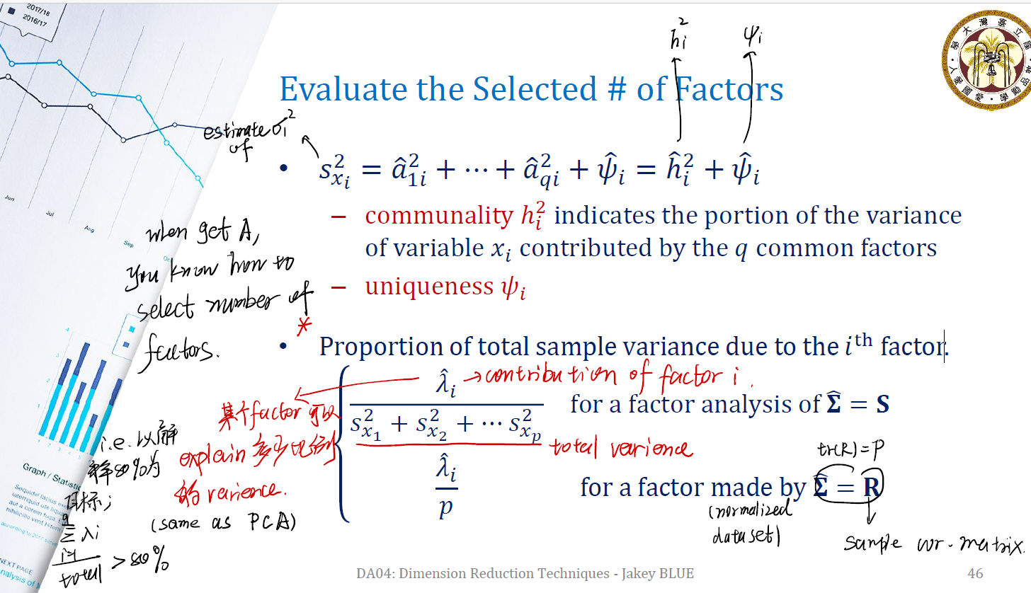
Evaluate the Selected # of Factors
$X$ 的样本方差为:
\[s_{xi}^2 = \hat{a_{1i}}^2 + ... + \hat{a_{qi}}^2 + \hat{\psi_i} = \hat{h_i^2} + \hat{\psi_i}\]- communality $h_i^2$ 表示 $q$ 个factor能解释 $x_i$ 多少比例的方差 ( indicates the portion of the variance of variable $x_i$ contributed by the $q$ common factors )。
- $\psi_i$ 是我们无法控制的方差。
所以,在筛选中,常常考察某一个 factor 可以解释多少比例的方差 ( Proportion of total sample variance due to the $i$ th factor ) 。解释方差比例为 $\hat{\lambda_i} / s_{x_1}^2 + … + s_{x_p}^2 $ 。
实际操作中,我们常常定一个比例。例如我们期望以 factors 能解释 $80\%$ 的总方差为目标,来分解 factors 。最后加总起来得到用哪一些 factors 来实现 dimension reduction 。
Examples of Factor Analysis (in AutoMPG dataset)
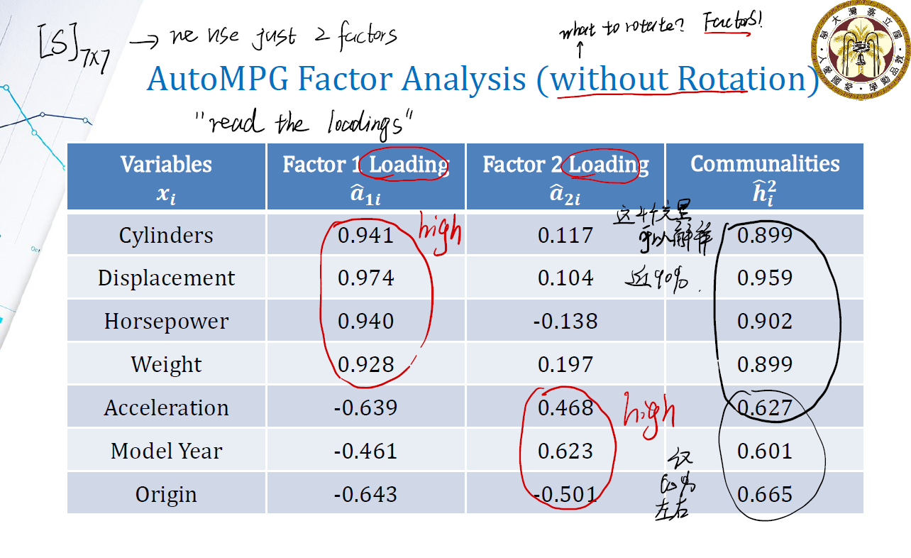
回想之前的“communality $h_i^2$ 表示 $q$ 个factor能解释 $x_i$ 多少比例的方差”。来看 communalities 这一栏:
- 分解出来的两个 factor ,对前面四个变量解释得不错,能解释几乎 $90\%$ 的方差。
- 对后面三个变量,只能解释大概 $60\%$ 的方差。
且,factor1 专注于解释前四个变量; factor2 专注于解释后面三个变量。
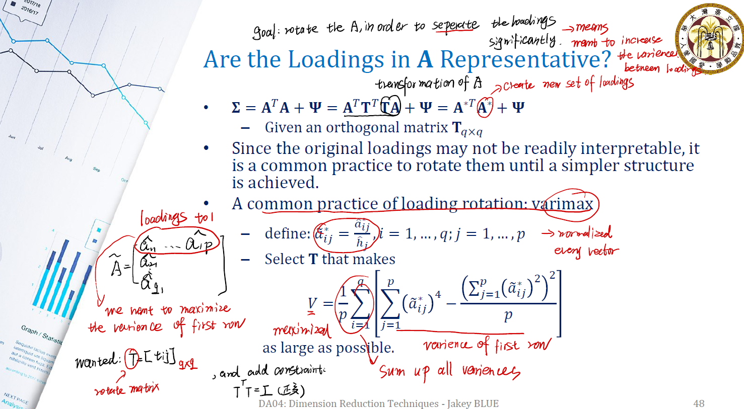
Are the Loadings in $A$ Representative ?
Our goal is: rotate the matrix $A$, in order to seperate the loadings significantly.
这意味着我们想增加 loadings 的方差。我们要对矩阵 $A$ 做一些变换。
依照之前的正交性,我们在分解协方差矩阵 $\Sigma$ 时,有:
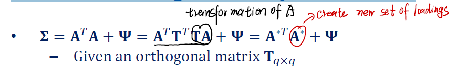
下面是一个经典的 rotate 方法:
After rotation … Revisit the original data set
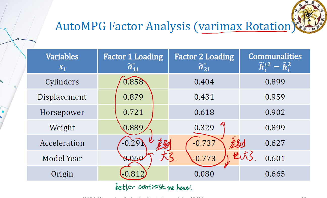
每个 factor 对应的 loading 差距增大了!这有助于我们识别出,哪一些变量对 factor 的影响较大。
Solving Factors
有了 loading matrix ,我们就可以用最小二乘的方法来拟合 factors 。
Effect of Rotation (loading matrix)
讲了这么多,让 loading matrix 的各个 loadings之间方差变大好处到底在哪里?看下面的这两幅图对比。
Without Rotation
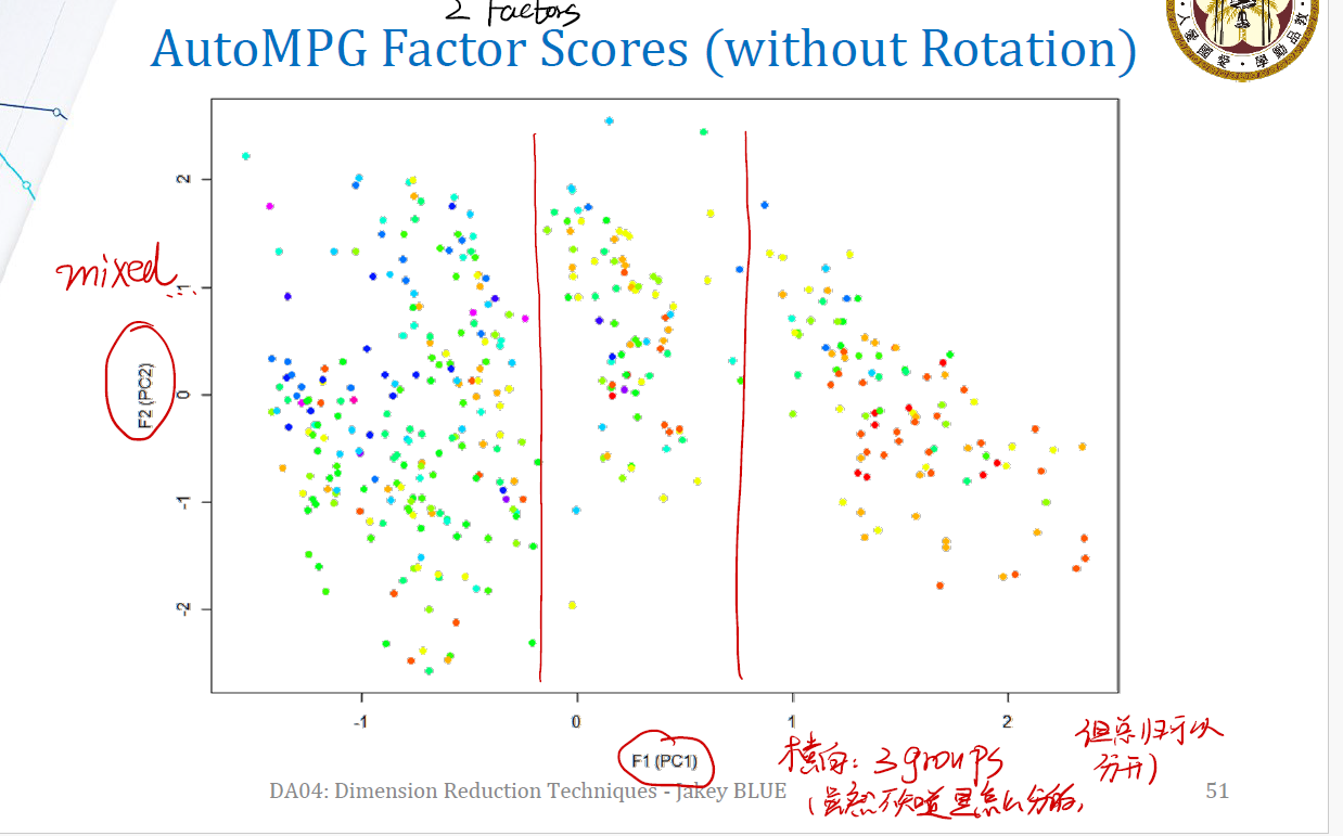
可以发现,从第一个 factor 的角度看,数据似乎可以分成三个部分。虽然不知道是怎么分开的,但是好像可以分开,也是不错的事情。
After Rotation
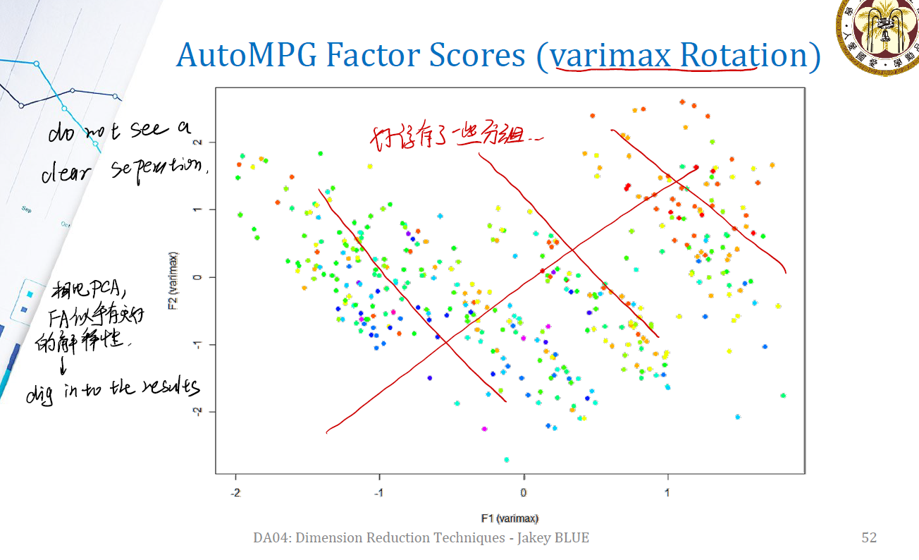
在做 rotate 后,从斜向来看,数据的分割更加明显,在两个 factor 上有了一些更加明显的分组。factors 能更好地解释哪些部分就更加明显了。
Reference
本文中的所有图片,Slides均来源于國立台灣大學工業工程學研究所藍俊宏副教授所開設的資料分析方法課程中之 DA04 Dimension Reduction.pdf。特此感謝藍俊宏老師在我學習歷程上的幫助!
In Covariance computing, we have $cov(AX) = Acov(X, X^T)A^T = Acov(X)A^T$, where $A$ is a constant vector. ↩︎