DA04 Dimension Reduction, Part II

DA04 Dimension Reduction :: Part II, Principal Component Analysis

In this note, we shall talk about the most popular and the most important technology in dimension reduction, which is, Principal Component Analysis.

What Does PCA Do?

PCA is a kind of transformation on the data set. In analysis, we always have an initial data set $X$. In PCA, we want to do a transformation, to transfer $X$ into $Z$, another data set with some constrains.

• Do what: Linearly transforming $p$ correlated variables into $p$ orthogonal basis. This means they are linear independent.
• Objective: Preserve the information in the data as much as possible.

We have a data set $X_{n \times p}$ , where $p \gg n$ . As we do not have enough data, we tend to pick up some important variables. In PCA, this is called feature extraction. And, PCA will create new features.

简单来说，PCA试图将数据集 $X$ 在某一系列的限制下，变成一个新的数据集 $Z$ 。并且尽可能多地保留原数据集 $X$ 中的信息。这也是一种投影。只不过我们是对数据集 $X$ 进行投影，让它投影到新的数据集 $Z$ 上。而在回归中，我们是对 $Y$ 进行投影，将其投影到 $X$ 的 column space 上。

Application: Dimension Reduction

• if # of variables $\gg$ # of observations, we can use PCA to reduce the dimension. In order to get enough data.
• or, we may encounter that some variables are highly correlated ( collinearity ). This means regression will not work. PCA can help us deal with it.

Example: Evaluate students

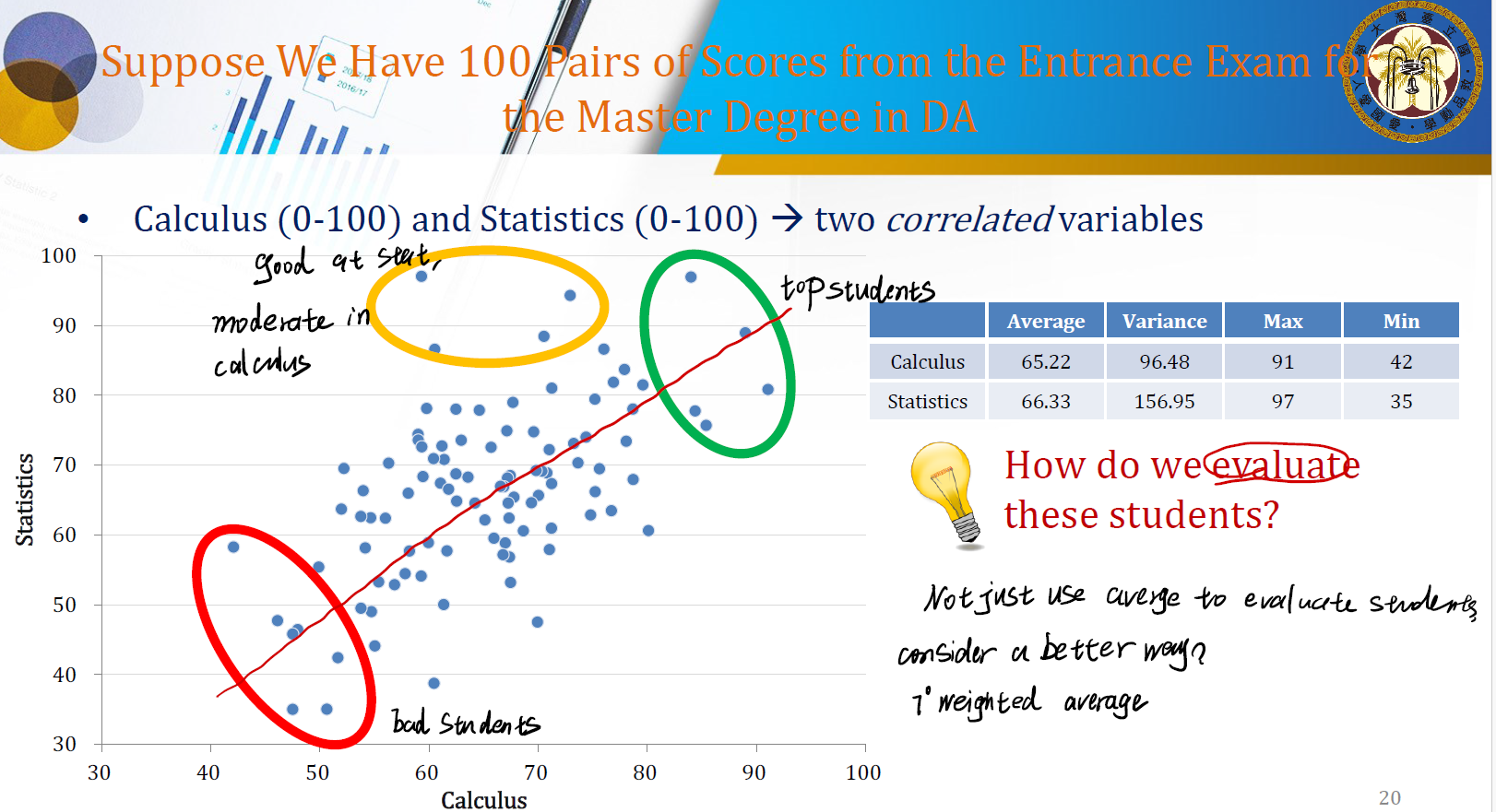
经常会遇到这种评估的情况。显然，如果两门都差一定是差生，两门都好一定是优生。但一门中等一门好，又该如何筛选呢？

Simple Average

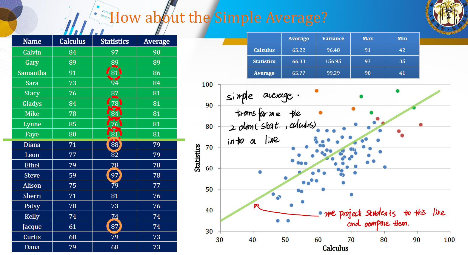
一个简单的想法是用均值来筛选。这也是一种投影。相当于将 stat 和 calculus 这两门的分数变成一条直线。然后将学生投影到这条直线上，进行比较。

Maybe… Another way?

我们的目标是要将学生筛选出来。很直观的一个感觉是，如果学生的分数之间方差越大，则越好筛选；方差越小，越难筛选。

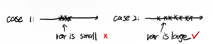
像这样，我们肯定希望是 case 2 的情形，我们能很清晰地找到数据之间的差异。一个很直观的方式是对 $X$ 进行 center:

\(X= \begin{gathered} \begin{bmatrix} X_C & X_S \end{bmatrix} \end{gathered} = \begin{gathered} \begin{bmatrix} X_{C1} & X_{S2} \\ X_{C2} &X_{S2} \\ \vdots & \vdots \\ X_{C100} & X_{S100} \end{bmatrix} \end{gathered}\) 然后，我们让 $X$ 中的每个数据都减去对应的 sample mean ，得到新的数据 $Z$ ：

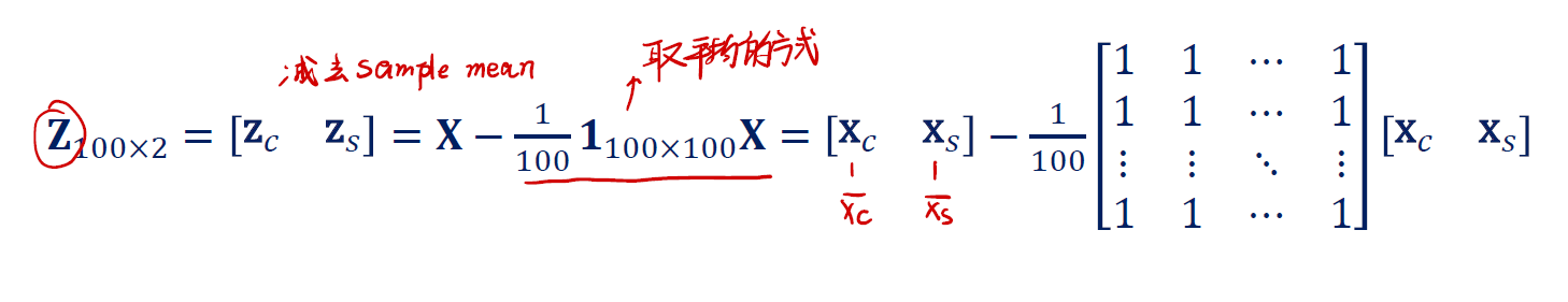
这样我们就得到了一个方差更大的新数据集。似乎，我们就能很好地分开数据并进行比较了。

Best Scatters Students

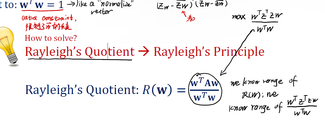
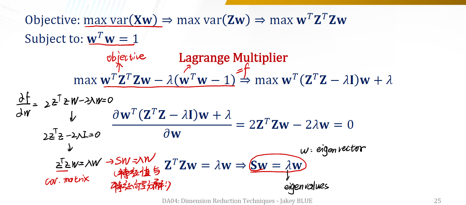
我们期望将 $X$ 通过投影 $w$ 制造出新的数据集 $Z$ ，并且极大化新的数据集 $Z$ 的方差。因此，我们的目标是：

\[\max var(Xw) \Rightarrow \max var(Zw) \Rightarrow \max w^TZ^TZw\]

并且，我们还要限制这个投影用的向量 $w$ 的长度（这类似于一种 “normalize vector” ）。subject to:

\[w^Tw = 1\]

为了解这样的一个最优化问题，我们有所谓的 Rayleigh’s Quotient 。

Rayleigh’s Principle

上面的 $R(w)$ 会被矩阵 $A$ 的第一个特征向量 $e_1$ 所极小化。并且， $R(w)$ 的最小值就是最小的特征值 $\lambda_1$ 。（ 注意矩阵 $A = Z^TZ$ ，也就是我们的新数据集 ）

最小值为：

\[R(w_1) = \frac {w_1^T A w_1} {w_1^Tw^1} = \frac {w_1^T \lambda_1 w_1} {w_1^Tw^1} = \lambda_1\]

Proof.

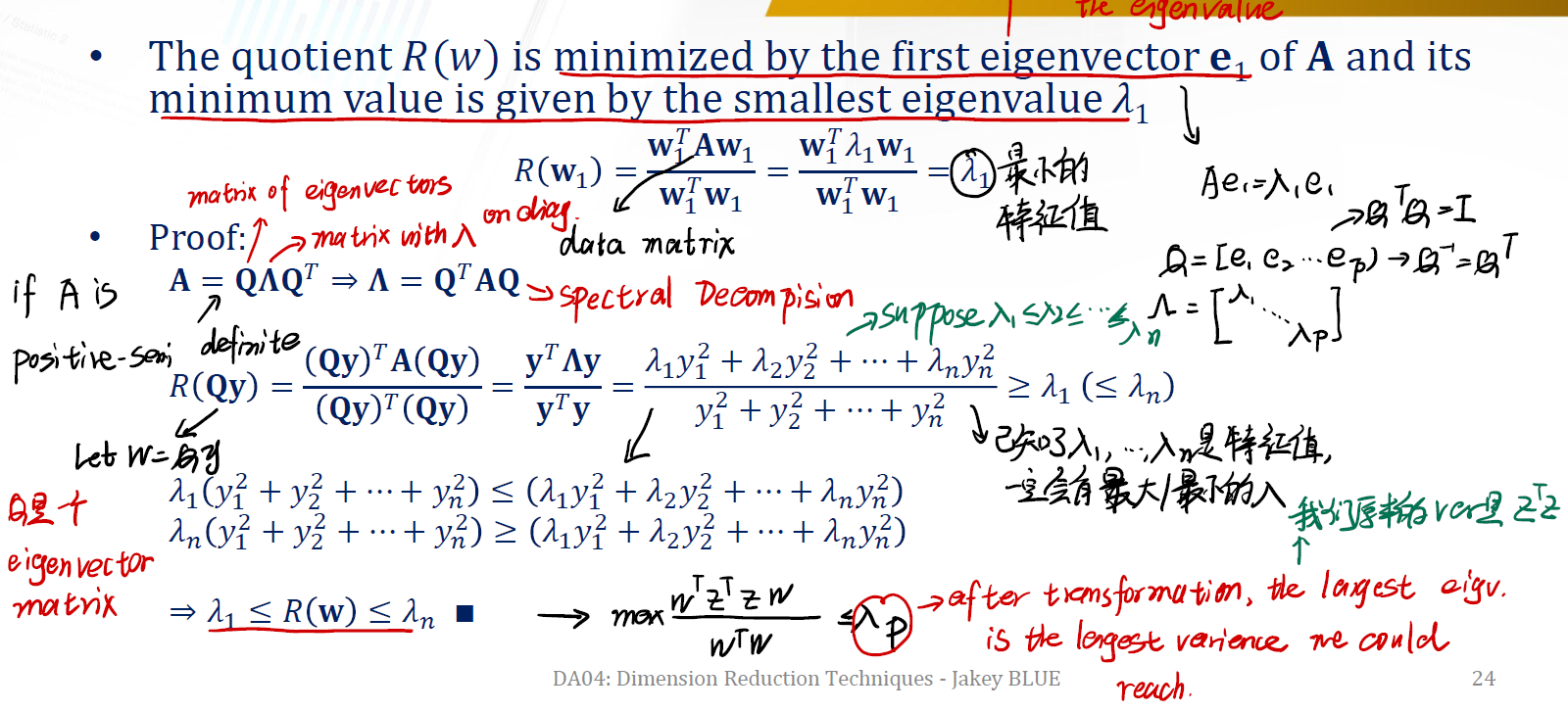
注意矩阵 $A$ 一定要是半正定矩阵。

Another Way to Find PCA Weights

同样可以使用 Lagrange Multiplier 来进行最优化过程。这次我们的目标是：

\(\max w^TZ^TZw - \lambda (w^Tw - 1) \Rightarrow \max w^T(Z^TZ - \lambda I)w + \lambda\) 然后我们对 $w$ 求偏微分，得到：

\[2Z^TZw - 2\lambda w = 0\]

解得：

\[Sw = \lambda w\]

这里的 $S$ 就是 covariance matrix 。而 $w$ 就是特征向量。

Preparing the Rayleigh’s Principle in Our Case

在我们的例子中，有：

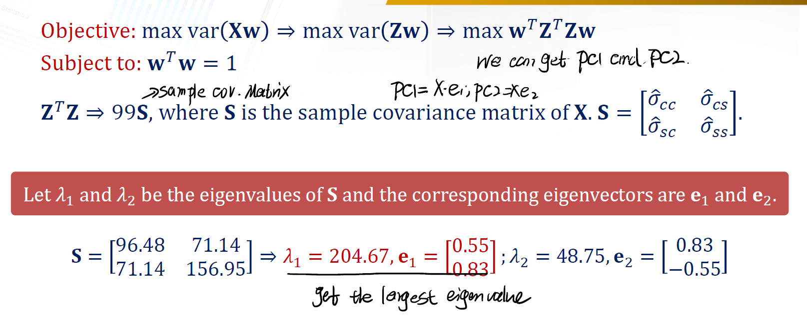
经过上面的一番运算，我们可以求得 sample covariance matrix 的两个特征值 $\lambda_1$, $\lambda_2$ 和其对应的特征向量。随后，我们就可以得到两个所谓的主成分 $PC_1$, $PC_2$ 。

Principal Component Extraction

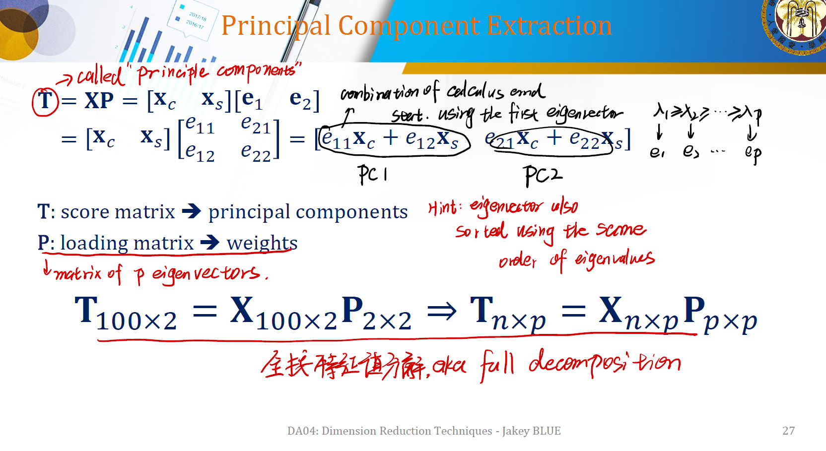
所以，我们的主成分又是怎么得到的呢？

我们先前想做的事情是将数据集 $X$ 通过一个矩阵 $P$ 做 transform，到一个新的数据集 $T$ 中。

\[T = XP = [X_C, X_S] [e_1, e_2]\]

其中 $e_1$ 和 $e_2$ 就是我们先前得到的两个特征向量。展开我们可以得到：

\[T = [e_{11} X_C + e_{12}X_S, e_{21} X_C + e_{22}X_S]\]

• 矩阵 $T$ 称为 score matrix ，这就是我们想找的 principal components。
• 矩阵 $P$ 称为 loading matrix ，由 weight 所组成。

在本例中，我们其实是将 $T$ 全部按照特征值进行了分解，即：

\[T_{n \times p} = X_{n \times p}P_{p \times p}\]

这种分解叫做 full decomposition 。

Properties of the Principal Components

我们得到的主成分也有一些独特的性质。

Variance Distribution

第一个主成分会有最多的 variance ，第二个主成分会有第二多的 variance，依次类推。

Proof.

\[Var(PC_1) = Var(Xe_1) = Var(Ze_1)\]

这里的 $Z$ 就是我们先前分数例子的数据。我们有：

\[Var(Ze_1) = E[(Ze_1)^T Ze_1] - E^2[Ze_1] = E[e_1^TZ^TZe_1] = E[e_1^TQ\Lambda Q^TZe_1]\]

其中，我们知道 $Z^TZ$ 就是 sample covariance matrix $S$ 。而我们可以做特征值分解：

\[S = Q \Lambda Q^T = \begin{gathered} \begin{bmatrix} 1 & 0 \end{bmatrix} \end{gathered} \times \begin{gathered} \begin{bmatrix} \lambda_1 & 0 \\ 0 & \lambda_2 \end{bmatrix} \end{gathered} \times \begin{gathered} \begin{bmatrix} 2 \\ 1 \end{bmatrix} \end{gathered}\]

带入后得：

\[Var(PC_1) = \lambda_1\]

同样地，也可以得到 $Var(PC_2) = \lambda_2$ 。

Fact 1. 每个主成分的方差是其对应特征向量的特征值。

Fact 2. 由 Fact 1. ，可以发现第一个主成分会有第一大的方差，第二个主成分有第二大的方差，以此类推。

Total Variance Maintains

分解的过程中，我们也有所谓的总方差保持性质，即：

\(V(X_c) + V(X_s) = V(PC_1) + V(PC_2) = \lambda_1 + \lambda_2\)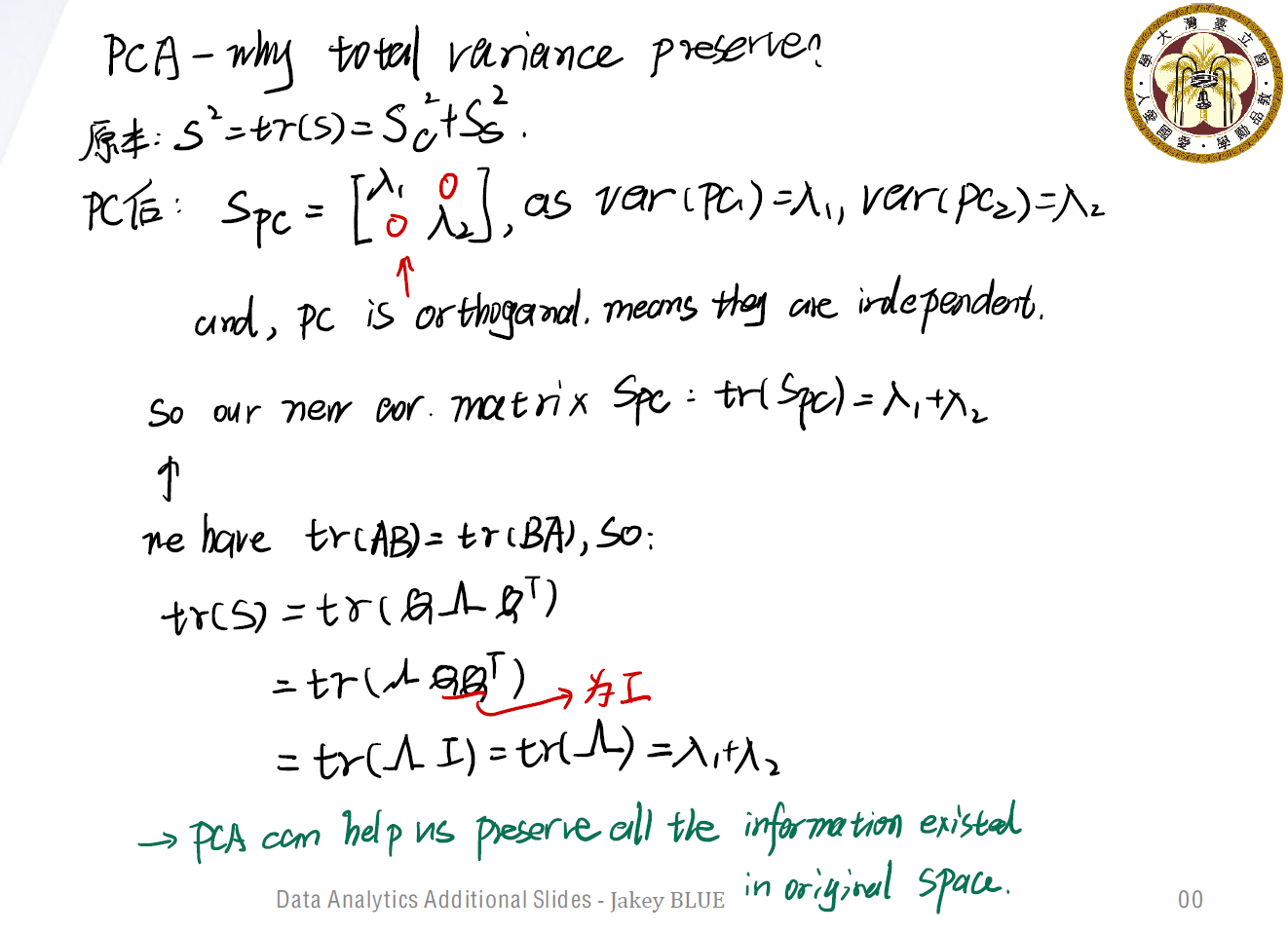

Independent Principal Components

每个主成分之间是互相线性独立的。

\[cov(PC_1, PC_2) = cov(Xe_1, Xe_2) = var(Ze_1, Ze_2) = E[e_2^TZ^TZe_1] = E[e_2^TQ\Lambda Q^Te_1] = 0\]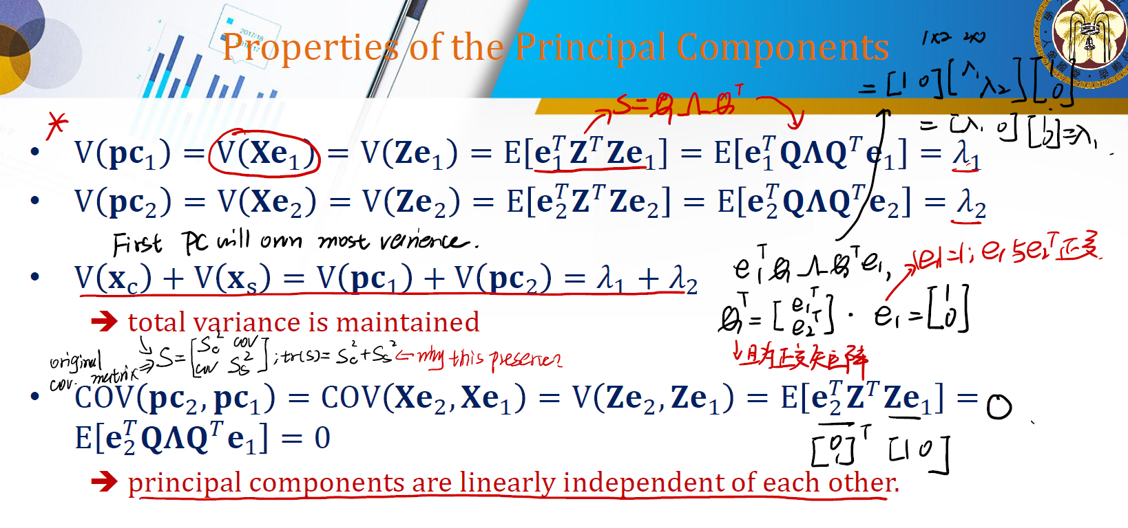

Geometric Meaning of PCA

现在我们来看PCA的几何意义。

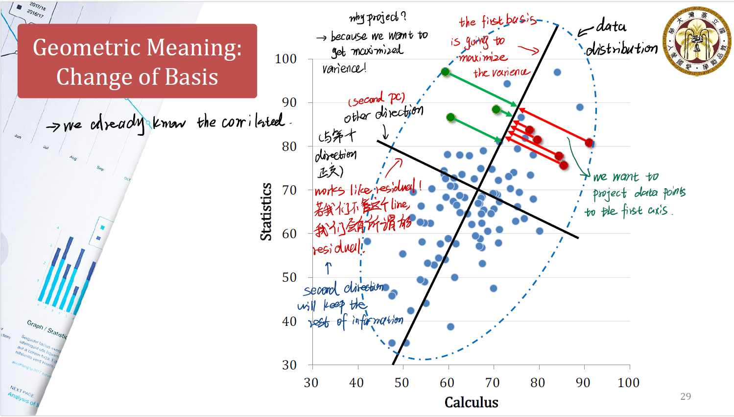
首先来看我们原本的情况。原本我们有一个 data distribution ，也就是上图中虚线框起来的部分。一开始我们试图用 Calculus 和 Statistics 两个维度来解释数据的分布情况。

先前我们提到，我们做的所谓主成分分析，其实就是对原本的 data distribution 做一个投影。因为我们想得到具有最大方差的数据。

在做 $PC_1$ 的投影时，我们将数据投影在斜向上的黑色线条上。这是我们分解出来的第一个主成分，又称为 first basis 。它将使得数据投影后的方差最大化。

在做 $PC_2$ 的投影时，我们当时期望向量正交，在这里也就是形成一个与第一个主成分方向正交的第二个主成分。这一个主成分会保留一部分余下的 information 。

这里很像回归分析中的 residual 。如果我们没有这个方向的分解，我们会有残差。正是这一个主成分协助我们保留下了第一个投影所无法涵盖的额外信息。

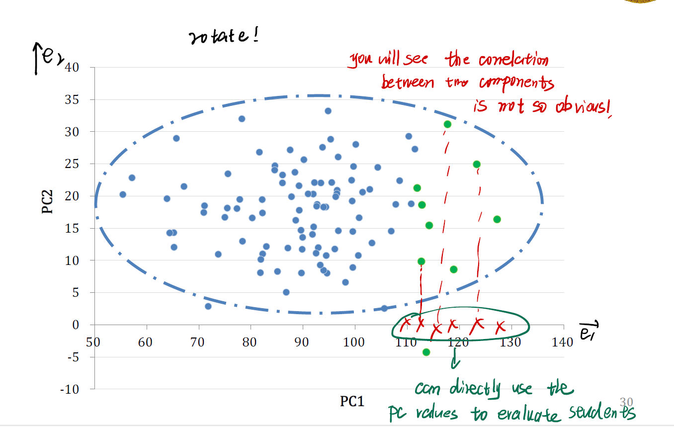
• 可以发现，如果我们再将数据按照 $PC_1$ 的大小排序，数据的区分变得更加容易了。
  • 我们可以直接使用 $PC$ 的值来评价学生的情况。
• 此外，数据之间的相关性也没有那么明显。

Why Relate PCA to Dimension Reduction

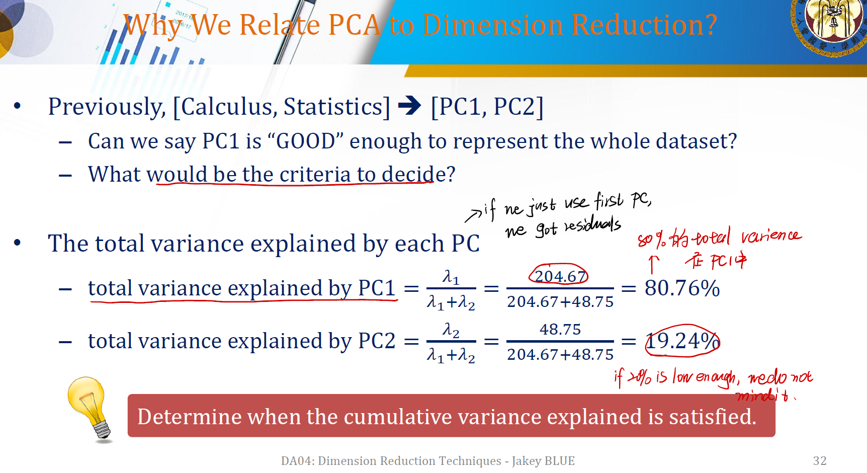
我们可以对每个主成分解释的方差比例进行分析。

第一个主成分解释了超过 $80\%$ 的方差，这意味着第一个主成分解释力较强。

PC1 is “GOOD” enough to represent the whole dataset, as it can explain nearly 80 percent variance of total variance.

Choose the # of Principal Components

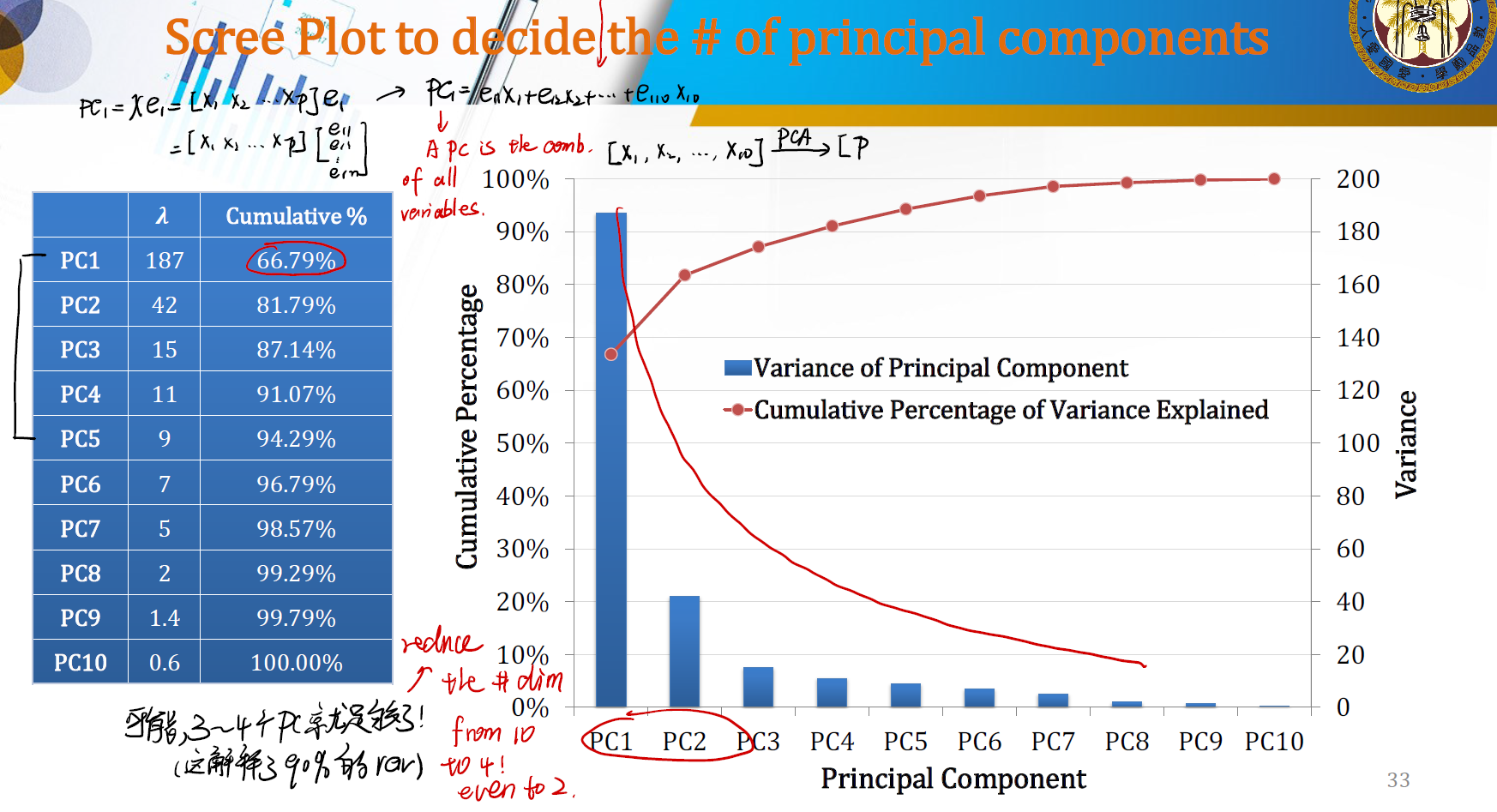
可以用方差的累计比例来计算我们到底需要多少个 PC 来进行分析。PC 的个数越少，就意味着我们 dimension reduction 的效果更明显。

例如，上图中我们可以选择 3~4 个 PC 。这将解释将近 90% 的信息，此外维度也从 10 降低到了 4 。

Explain the result

当然不能只用主成分来说明，还要回归到主成分是被那些变量组装起来的。

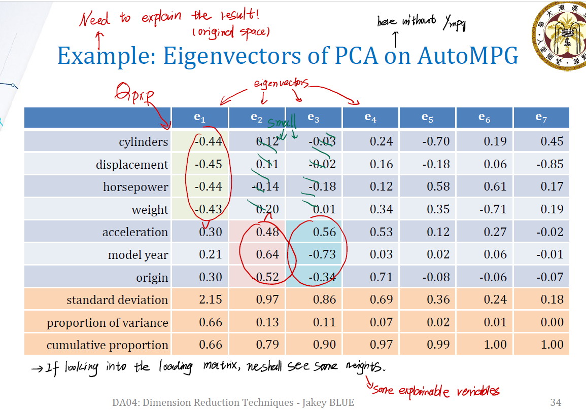
例如，上图中我们很明显能发现，第一个主成分对应的特征向量 $e_1$ 歧视主要由前四个 variable 构成，第二个主成分和第三个主成分主要由 acceleration, model year, origin 这三个 variable 构成。

这就可以解释我们的分析过程。

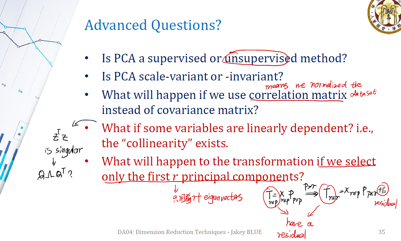
Advanced Questions