DA03 Multivariate Statistical Inference
DA03 :: Multivariate Statistical Inference
In this section, we will continue delving into multivariate statistical inference.
Random Matrix, Vector, and Variable
Let’s review some mathematical definitions and marks.
$X$ is a random variable and $x_1, x_2, …, x_n$ are the $n$ observations of a random sample from $X$.
We have Sample average:
\[\bar{x} = \frac {1} {n} \sum_{i = 1}^n x_i\]and we have Sample variance:
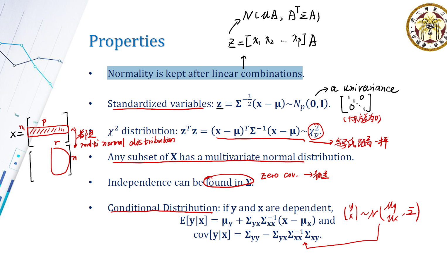
\[s^2 = \frac {1} {n - 1} \sum_{i = 1}^n (x_i - \bar{x})^2\]In Matrix Form, assume we have $p$ random variables and $n$ observations of each random variables. we can express the random sample as:
\[X_{n \times p} = \begin{gathered} \begin{bmatrix} x_1 & x_2 & \dots & x_p \end{bmatrix} \end{gathered}\]In this case, $x_1, x_2, …, x_p$ are $n \times 1$ column vectors. We can expand them:
\[X = \begin{gathered} \begin{bmatrix} x_{11} & ... & x_{1p} \\ \vdots & \vdots & \vdots \\ x_{n1} & \dots & x_{np} \end{bmatrix} \end{gathered}\]and, we always have $n » p$. The number of rows means we have $n$ observations, and the number of columns means we have $p$ variables. And, this $n » p$ means we have much more data than variables.
Sample Mean and Variance of Matrix $X$
So we need to know how to calculate sample mean and sample variance when we have matrix data.
Sample mean
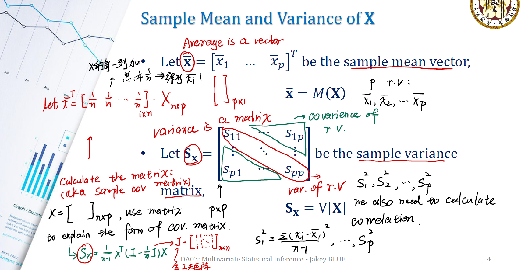
Let $\bar{x} = [\bar{x_1}, \bar{x_2}, …, \bar{x_p}]^T$ be the sample mean vector. This can also in Matrix form:
\[\bar{X}^T = \begin{gathered} \begin{bmatrix} \frac {1} {n} & \frac {1} {n} & ... & \frac {1} {n} \end{bmatrix} \end{gathered}_{1 \times n} \times X_{n \times p}\]这就是将矩阵 $X$ 的每一列加总乘以 $1/n$ ,从而得到相应的 $\bar{x_i}$ 。
要注意, $\bar{x_i}$ 是一个 $p \times 1$ 的列向量。
Sample Variance
在矩阵形式的 sample 下,样本方差也是一个矩阵。可记为:
\[S_x = \begin{gathered} \begin{bmatrix} s_{11} & \dots & s_{1p} \\ \vdots & \ddots & \vdots \\ s_{p1} & \dots & s_{pp} \end{bmatrix} \end{gathered}\]在这个样本方差矩阵中,要注意的是。对角线上的是对应变量的方差,而 $s_{ij}$ 是变量 $i$ 与变量 $j$ 的协方差。我们也可以将其写作矩阵运算的形式:
\[S_x = \frac {1} {n - 1} X^T(I - \frac {1} {n} J) X\]其中,矩阵 $J$ 是一个 $n \times n$ ,且内部元素全为 1 的矩阵。
Sample Correlation of $X$
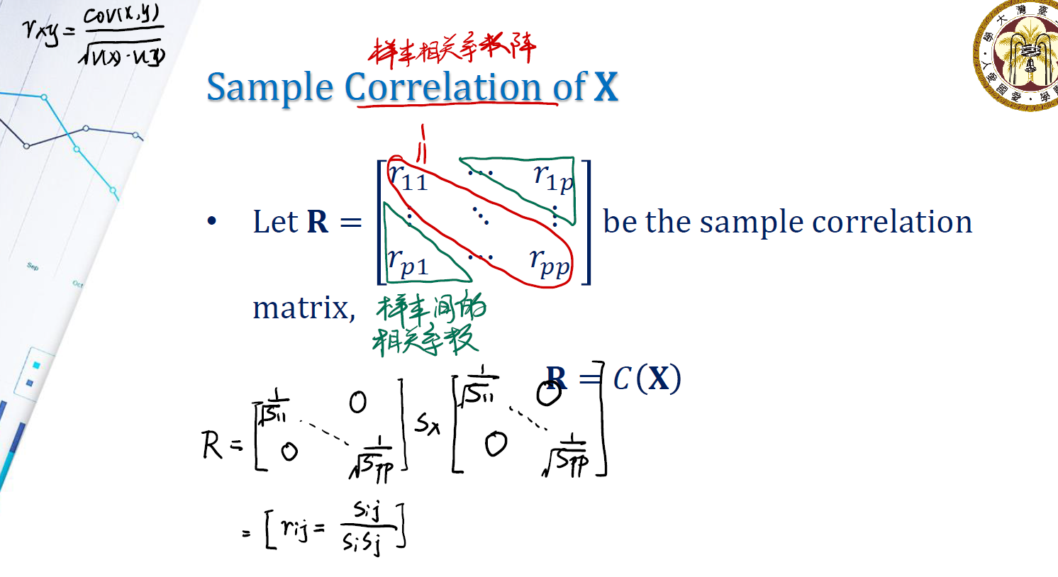
让我们来看一下样本相关系数矩阵。
\[R = \begin{gathered} \begin{bmatrix} r_{11} & \dots & r_{1p} \\ \vdots & \ddots & \vdots \\ r_{p1} & \dots & r_{pp} \end{bmatrix} \end{gathered}\]其中, $r_{ij}$ 是变量 $i$ 和变量 $j$ 之间的相关系数。相关系数的计算公式为:
\[r_{xy} = \frac {cov(x, y)} {\sqrt{var(x) var(y)}}\]同样地,也可以用矩阵运算的形式来表示。
\[R = \begin{gathered} \begin{bmatrix} \frac {1} {\sqrt{s_{11}}} & \dots & 0 \\ \vdots & \ddots & \vdots \\ 0 & \dots & \frac {1} {\sqrt{s_{pp}}} \end{bmatrix} \end{gathered} \times S_x \times \begin{gathered} \begin{bmatrix} \frac {1} {\sqrt{s_{11}}} & \dots & 0 \\ \vdots & \ddots & \vdots \\ 0 & \dots & \frac {1} {\sqrt{s_{pp}}} \end{bmatrix} \end{gathered}\]其中有 $r_{ij} = \frac {s_{ij}} {s_is_j}$ 。
Linear Transformation of $X$
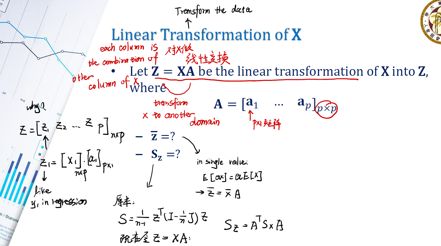
在线性代数中,我们知道矩阵相乘就是一种线性变换。用于做乘法的矩阵是一个函数,将在一个线性空间 $\mathbb{R}^n$ 中的矩阵映射到另一个线性空间 $\mathbb{R}^m$ 中。
在 regression 中,我们也有对 dataset 进行线性变换的需求。因此我们也会需要相应的变换矩阵。
\[Z = XA\]是一个将 $X$ 变换到 $Z$ 的线性变换。其中,
\[A = \begin{gathered} \begin{bmatrix} a_1 & \dots & a_{p} \end{bmatrix} \end{gathered}_{p \times p}\]我们可以算出变换后的新 dataset 的样本均值与样本方差。
\[\bar{Z} = \bar{X} A\] \[S_z = A^TS_xA\]可以发现,矩阵 $Z$ 中的每个 column 都是原本矩阵 $X$ 的每个 column 的线性组合。
Overall Variability of $X$
Here are several special matrix statistics we need to introduce.
Generalized Sample Variance of X
这是所谓的 样本广义方差,计算方式为对样本方差矩阵 $S_x$ 取行列式值。用来描述数据的稀疏性( sparsity )。
Total Sample Variance of X
这是总样本方差。就是把每个变量的自身方差相加。即:
\[\sum_{i = 1}^p S_{ii}\]这也是样本方差矩阵 $S_x$ 的 trace。即 $tr(S_x)$ 。
这个方差会有一点高估总体的 information 。因为很可能在 $x_1, x_2, …, x_p$ 中,有一些变量之间有相关性,它们的方差不能简单地加减。举例来说,如果 $x_1$ 和 $x_2$ 呈现高度相关,将其方差直接相加必然有高估( inflating)。
Distance between Vectors
接下来要介绍的是如何判断两个 vector 之间的距离。这是一个很重要的观念。
Euclidean Distance
我们最常用的是欧氏距离。计算公式为:
\[\sqrt{(X_1 - X_2)^T(X_1 - X_2)}\]但在数据集中,欧氏距离真的合理吗?看下面的这个例子。
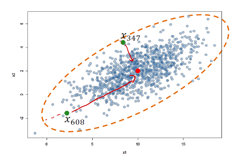
出现了一个很奇怪的现象:
- 按照欧氏距离的定义,向量 $x_{347}$ 相较于中心点(红色点)显然比向量 $x_{608}$ 更加接近。因此,似乎 $x_{347}$ 更接近数据分布的中心。
- 但如果我们关注数据集的分布。很显然,越靠近边缘,意味着数据点离数据集分布中心越远。显然的是, $x_{347}$ 相对于 $x_{608}$ 更靠近边缘。欧氏距离给出了一个错误的结果。
我们需要另一种距离的测定方式,来断定 sample 距离数据集中心到底有多远。
Mahalanobis Distance
马氏距离通过考虑两个向量之间协方差的方式,有效地刻画了在一个数据集中向量距离数据集中心的远近。马氏距离同样也考虑了数据的 distribution 。其计算公式为:
也可以写成矩阵的形式:
\[\begin{align*} \text{Mahalanobis Distance} & = \sqrt{(\bar{x} - \mu_x)^TS^{-1}(\bar{x} - \mu_x)} \\ & = \sqrt{(\bar{x} - \mu_x)^T\Sigma^{-1}(\bar{x} - \mu_x)} \end{align*}\]其中,
- $\bar{x}$ is the
sample meanvector. - $\mu_x$ is the
real meanvector. - $S^{-1}$ is the
sample covariance matrix. - $\Sigma^{-1}$ is the
real covariance matrix.
Equation above tells us how far the sample mean vector to the real mean vector (aka real center).
Multivariate Normal Distribution
Now let’s introduce the Multivariate Normal Distribution.
In Univariate Normal Distribution, we have already known,
And, in Multivariate Normal Distribution, we have:
where,
- $\Sigma$ is the
covariance matrix. This is one argument we need to estimate. - $\mu$ is the
mean vector. This is another argument we need to estimate.
在协方差矩阵中,每两个参数就要求协方差。总共有 $C_p^2$ 个未知变量要估计;在均值向量 $\mu$ 中,有 $p$ 个均值要估计,此外,还要计算 $p$ 个样本方差 所以,总共加起来有 $(2p + C_p^2)$ 个待估计参数。
Properties
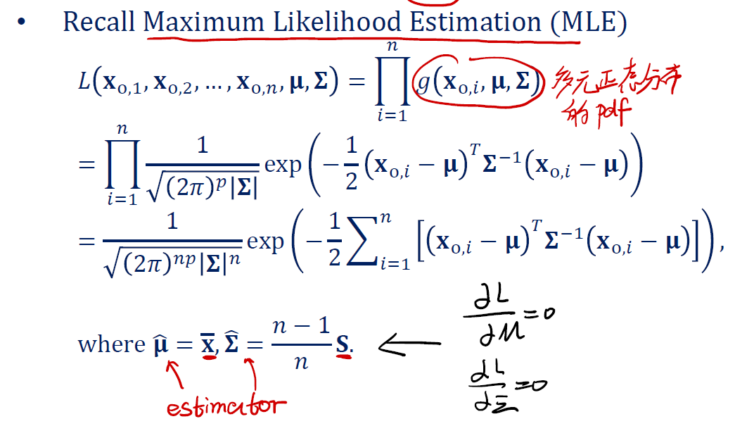
Multivariate Normal Estimates
可以利用极大似然法进行参数的估计。
Distribution of $\bar{x}$ and $S$
我们已经知道了 $\bar{X} = \sum_{i = 1}^n \frac {1} {n} X_{o, i}$ ,且 $x_{o, i} \sim N_p(\mu, \Sigma)$ 。因此有,
\[\bar{x} \sim N_p(\mu, \frac {\Sigma} {n})\]此外,样本协方差矩阵 $S$ 服从 Wishart distribution ,经过转换可以得到多元卡方分布。
Multivariate Hypothesis Testing with $\Sigma$ Known
在假设检验时,我们要检验多个参数。显然不能一个个检验,否则 Type I error 将会飙升。
我们希望同时检验是否有 $\mu_1 = \mu_2 = … = \mu_p$ 。因此,假设检验为:
\[H_0 : (\mu_1, ..., \mu_p )^T = (\mu_{01}, ..., \mu_{0p})\]采取的检定统计量为:
\[Z^2 = n(\bar{x} - \mu_0)^T\Sigma^{-1}(\bar{x} - \mu_0)\]这个统计量服从 $\chi_p^2$ 分布。
如果 $Z^2 > \chi_{\alpha, p}^2$ ,则拒绝原假设 $H_0$ 。
Hotelling’s $T^2$-Test with $\Sigma$ Unknown
当然也有 $\Sigma$ 未知的情况。我们要用一个新的检定统计量 $T^2$。
\[T^2 = n(\bar{x} - \mu_0)^T S^{-1} (\bar{x} - \mu_0) \sim T^2_{p, n - 1}\]其中,我们用样本协方差矩阵 $S$ 来替代总体协方差矩阵 $\Sigma$ 。
这个分布与 F-distribution 有关。
\[T_{p, n - 1}^2 = \frac {p(n - 1)} {n - p} F_{p, n - p}\]如果 $T^2 > T^2_{\alpha, p, n - 1}$ ,拒绝原假设 $H_0$ 。
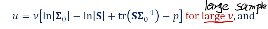
Test of Covariance Matrix
接下来的问题自然很明确,我们得到了一个协方差矩阵的估计 $\Sigma_0$ 。我们要观察它是否与真正的协方差矩阵有显著差异。我们有两个统计量。
在有大量的 sample 下,我们要使用的统计量是:
在适中/小样本的情况下,我们使用的统计量是:
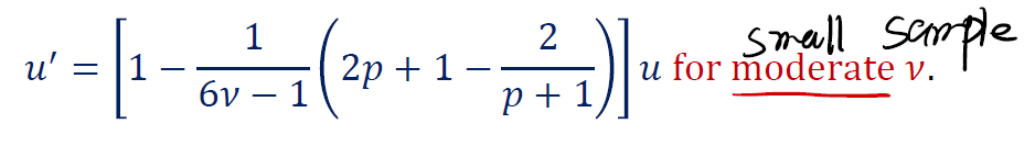
其中,$\upsilon = n - 1$ ,是 $S$ 的自由度。
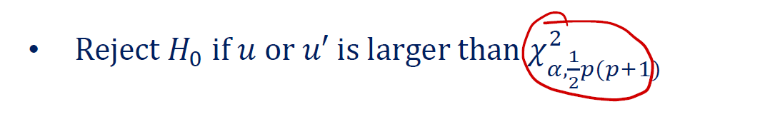
拒绝域是:
在多元中,还有很多的 test 。这里不一一给出。
Multivariate Analysis of Variance (MANOVA)
现在我们面临的一个问题自然是,如何在多元的情况下开展 ANOVA 分析?
Review of All sorts ANOVA
所谓的“方差分析”并不是真正的分析方差!而是比较 mean vectors ,从而达到一个检定,检验多个的效果。
We want to know how different levels will impart our response.
在 ANOVA 时,我们通常认为 response $y_{ij}$ 被几个因素所影响:
- mean
- levels
- some residual $\epsilon_{ij}$, this is which we can not control
分析的目标就是,鉴定是否是
levels影响了我们的 response ?
One-way ANOVA
我们熟悉的是所谓的 one-way ANOVA 。我们做 $n$ 次重复实验,总共有 $a$ 个 level 。检验表达式为:
\[y_{ij} = \mu + \tau_i +\epsilon_{ij}, \text {where } i = 1, ..., a; j = i, ..., n\]Multi-way ANOVA
在 Multi-way ANOVA 中,我们想要检验是否有多个因素影响了我们的 response 。以两个因素影响为例:
\[y_{ijk} = \mu + \tau_i + \gamma_j + \epsilon_{ijk}\]其中, $i = 1, …, a$ ;$j = 1, …, b$ ; $k = 1, …, n$ 。这意味着第一个 factor 有 $a$ 种 level ,第二个 factor 有 $b$ 种 level ,总共观测了 $n$ 笔资料。
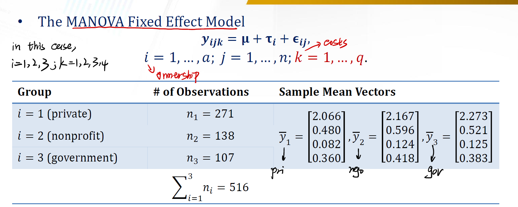
MANOVA
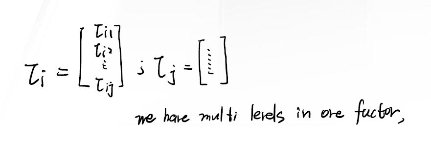
在 MANOVA 中,我们的 level 不是一个数值了,而是一个 vector 。
\(y_{ijk} = \mu + \tau_i +\epsilon_{ijk}\) 其中, $i = 1, …, a$ ; $j = 1, …, n$ ; $k = 1, …, q$ 。意味着我们有 $q$ 个 random variable ,$a$ 种 level , $n$ 笔观测资料。
当然还是不能拆分成 multiple one-way ANOVA 。会有 Type I error inflation 。
Compare to Regression Analysis
- $\tau$ 代表的是 level ,有固定值如 $1, 2, 3, 4$ ;而回归分析中 $x$ 是一个随机变量,有多个不同的值。
- 在 ANOVA 中,我们假设 response (也就是 y )被 level 影响。我们想要知道 level 能影响多少。
Analysis Of Variance (ANOVA, uni-variate case)
What if I got categorical predictors?
我们通过一个例子来了解 ANOVA 的流程以及意义。
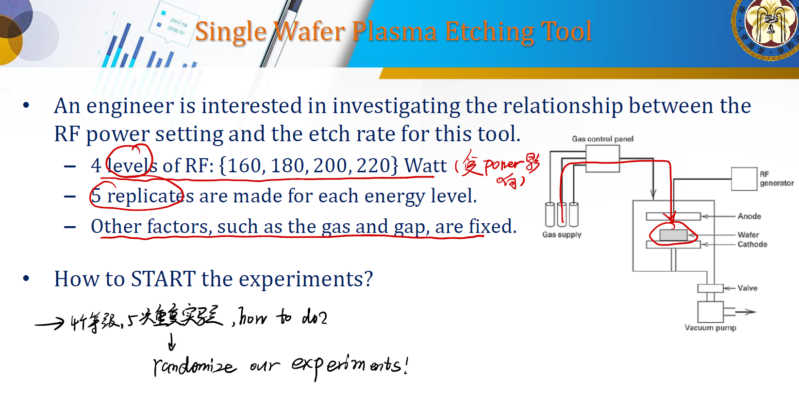
- 我们要研究的 response 是
etch rates,我们的 level 是RF。有四个可能值 ${160, 180, 200, 220}$ 。 - 在每个 level 中,我们都做 5 次重复实验。
- 其他的影响因素都是定值。
怎么开始实验? $\longrightarrow$ 很显然,我们要做所谓的 randomize 。
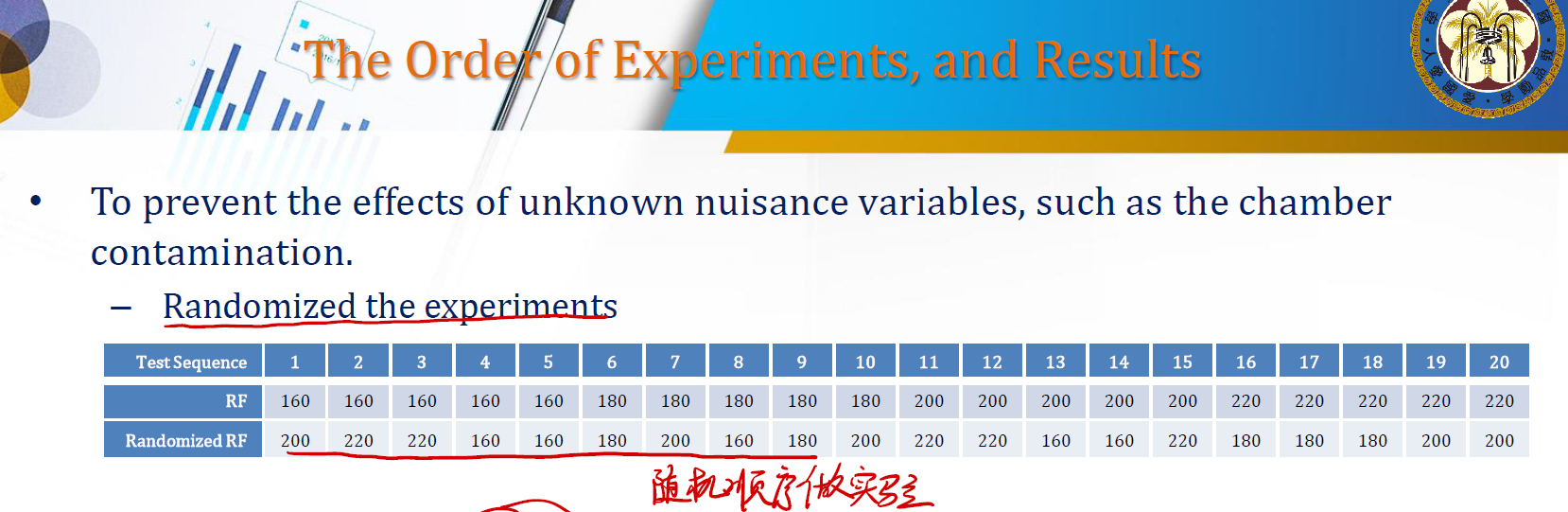
Start of Experiments
为了防止其他的未知影响,我们要随机进行实验。只要控制好 level 和每个 level 的重复次数即可。
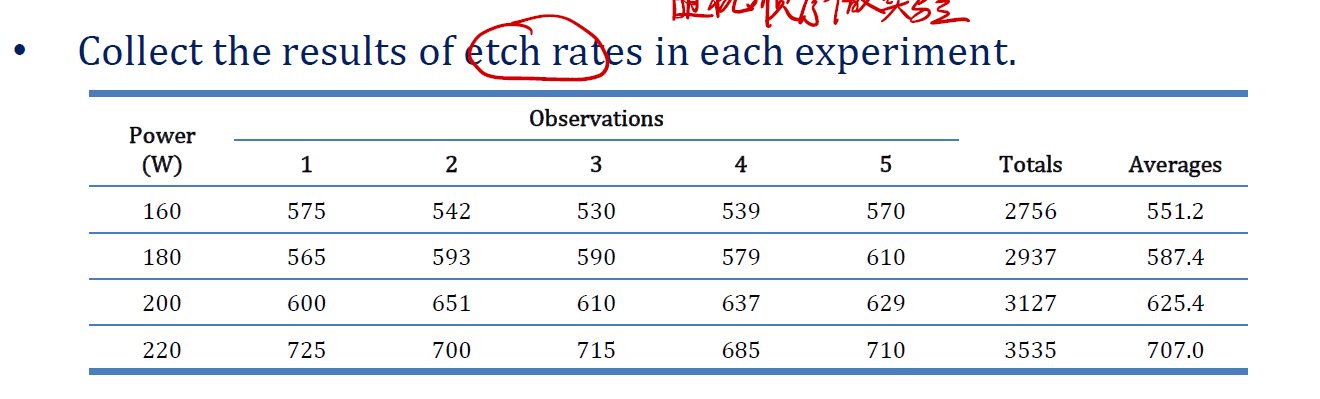
随后,可以分别对每个 level 的观测值加总,取均值得到我们想要的 etch rates 。
Data Visulization
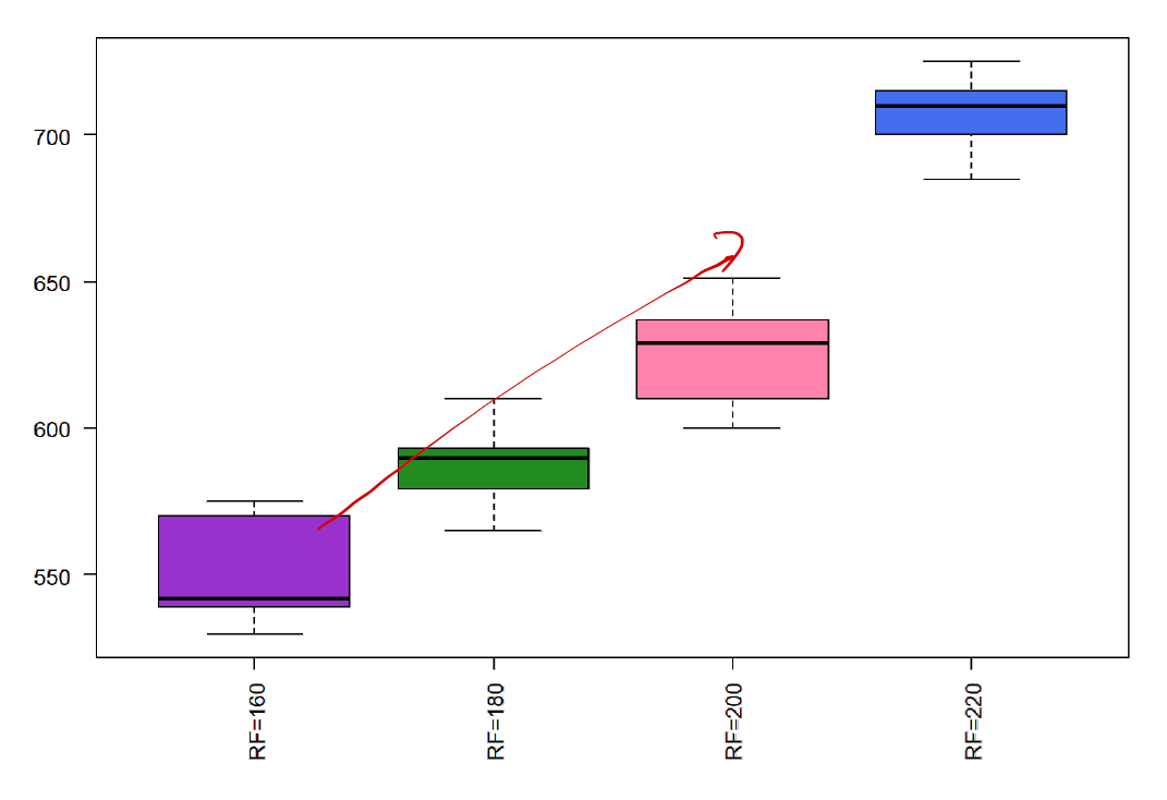
最直观的方式是通过箱线图来展示不同 level 的相关影响。我们可以看到,似乎随着 level 的增加, rate 呈现一个上升趋势。且每一个箱体之间都能很好地分别。
但这只是最直观的感觉。我们真的能说:
- RF power setting affects the etch rate?
- higher RF results in increased etch rate?
如果我们要做 t-test ,这是一件非常痛苦的事情。比如,我们要证明 $\mu_{180} > \mu_{160}$,也要证明 $\mu_{200} > \mu_{160}$ 。总共要做 $C_4^2$ 次 t 检验。这不但很繁琐,而且会导致 Type I error inflating 。
这个时候就要请出我们的 ANOVA 了。用来一口气检查 RF power factor 是否真的影响我们的 etch rate 。
Fixed or Random Effects Model
首先明确我们检测的到底是什么:
- 我们检测的目标是判断 RF level 会有什么样的影响。
- response 是 etch rate ,effect 是 RF level 。
做 ANOVA 分析,我们可以构建两种 model 。一种是所谓的 means model ,将 level 合并到均值来检测。一种是 effects model ,单独将 level 拿出来检测。
其中, $i$ 是所谓的 treatement ,即多少个 level 。而 $j$ 是 replicate ,即实验重复多少次。
这里的 $\mu_i$ 是均值 $\mu$ 和 effect $\tau_i$ 之和。
在 effects model 中,我们的检测表达式是:
\[y_{ij} = \mu + \tau_{i} + \epsilon_{ij}\]其中, $i$ 是所谓的 treatement ,即多少个 level 。而 $j$ 是 replicate ,即实验重复多少次。不过在这个形式中,我们只关心 $\tau_i$ 。
此外,在检定过程中,我们的假设是:
\[y_{ij} \sim N(\mu + \tau_i, \sigma^2)\]不过这个假设有的时候可以忽略。毕竟很难有服从正态分布的情况发生。
Analysis of the Fixed Effects Model
现在我们要分析 fixed effects model 。我们的假设是:
\[H_0 : \mu_1 = \mu_2 = \dots = \mu_a \\ H_1: \mu_i \neq \mu_j \text{ for at least one pair } (i, j)\]这个条件的意思是,所有的 treatment 中资料的均值都一样。这意味着, $\tau_i$ 并没有影响均值,也就印证了其没有影响我们的 response $y$ 的值。
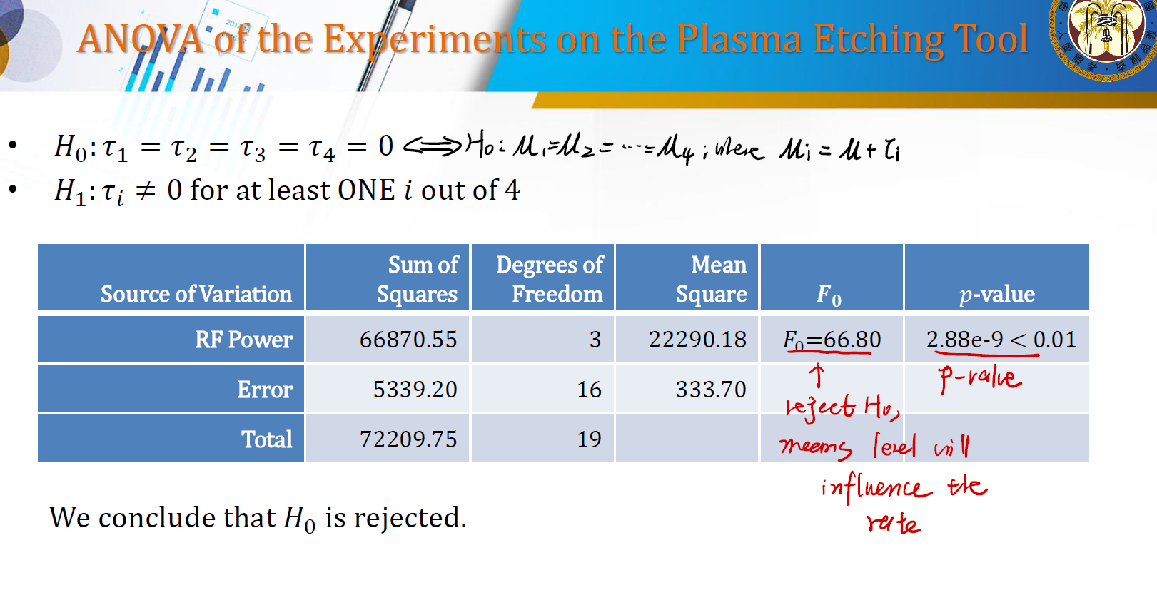
如果我们采用的是 effects model ,我们有与之等价的假设:
\[H_0 : \tau_1 = \tau_2 = \dots = \tau_a = 0 \\ H_1 : \tau_i \neq 0 \text{ for at least one } i\]这个假设的意思是,所有 $a$ 个 effects 是一样的吗?如果是一样,则 treatment 对 response 几乎没有影响。
The Decomposition of the Total Sum of Squares
现在要进行经典的任务:对 Total Sum of Square 进行分解。首先我们明确两组记号:
\[\bar{y}_{..} = \sum_j \sum_i y_{ij} \times \frac {1} {a_n}\]上式表示的是所谓的 overall mean ,即所有抽取的资料的均值。
上式表达的意思是,给一个固定的 $i$ (即将 treatment 固定),求取平均值。这个求的是某个 treatment 下的样本平均值。( Sample Average of Certain Level )
下面我们来对 Total Sum of Square 进行分解。
\[\begin{align*} SS_T & = \sum^a_{i = 1} \sum^n_{j = 1} (y_{ij} - \bar{y}_{..})^2 \\ & = n\sum^a_{i = 1} (\bar{y}_{i.} - \bar{y}_{..}) ^ 2 + \sum^a_{i = 1} \sum^n_{j = 1} (y_{ij} - \bar{y}_{i.})^2 \\ & = SS_{\text{treatment}} + SS_{E} \end{align*}\]我们可以将 Total Sum of Square 分成两部分。
- 第一部分是每一个 treatment 组的均值减去所有样本加总的SS,称为
组间均值 SS( between level/group )。 - 第二部分是组内的 observation 和 certain level mean 相减并加总的SS,称为
组内差值 SS(within level/group SS )。
在分解完毕后,我们可以得到一张 ANOVA Table :
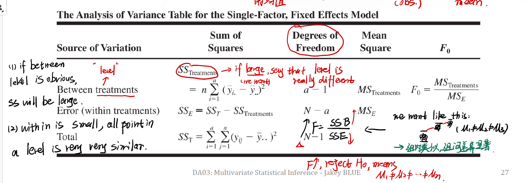
- 在整体中,方差来源于三部分:
Between treatment:不同 level 导致的方差。这就是上面提到的 SS-treatment 。它刻画了不同 level 之间是否有不同。这个越大,说明每个 level 确实会导致 response 之间的不同。 (这也是我们想要利用ANOVA证明的结果,即 treatment 真的会对 response 有影响)Error (within treatment):这是每个 treatment 内的不同。是所谓的组内差值(差异)。刻画了每个 treatment 组内数据的差异。如果 within is small ,则可以证明在同一个 level 中的数据点 point 非常的 similar
- 我们希望达到的结果是:组内的数据点都类似,组间的数据都有很显著的差异。就像我们之前的箱线图一样。
我们使用的检定统计量是 F 。在这里,$F = SS_{\text{between}} / SS_E $ 。如果 $F \uparrow$ ,则我们有充足的理由拒绝原假设 $H_0$ ,说明 level 对 response 的影响是显著的。这也是组间差异 SS-between 增大 ,组内差异 SS-Error 减小而的来的结果。
When the effects are in vectors : Multivariate Analysis Of Variance (MANOVA)
如果我们发现,所谓的 effect $\tau$ 现在不是一个单纯的 level 值了,而是一个 vector 。我们又怎么进行方差分析呢?这就是要使用 MANOVA 的时候。
The Hypothesis of MANOVA
我们的原假设是:
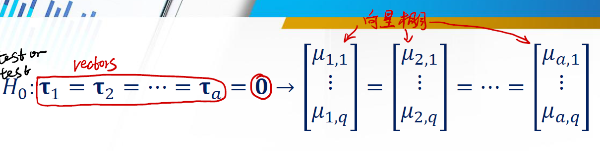
这里的 $\tau$ 都是 vector ,而非之前的标量。我们希望检测,这些向量是相同的。之前我们的 $SS_{\text{between}}$ 和 $SS_E$ 也不再是一个标量,而变成矩阵。
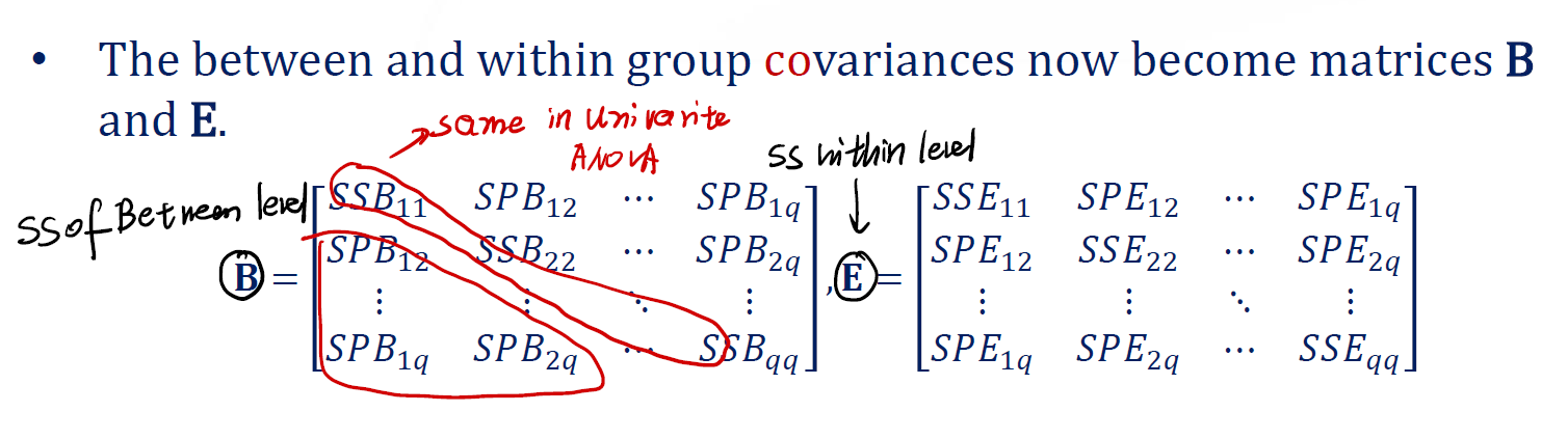
矩阵 $\mathbf{B}$ 代表着 SS of between level ,而矩阵 $\mathbf{E}$ 代表着 SS within level 。
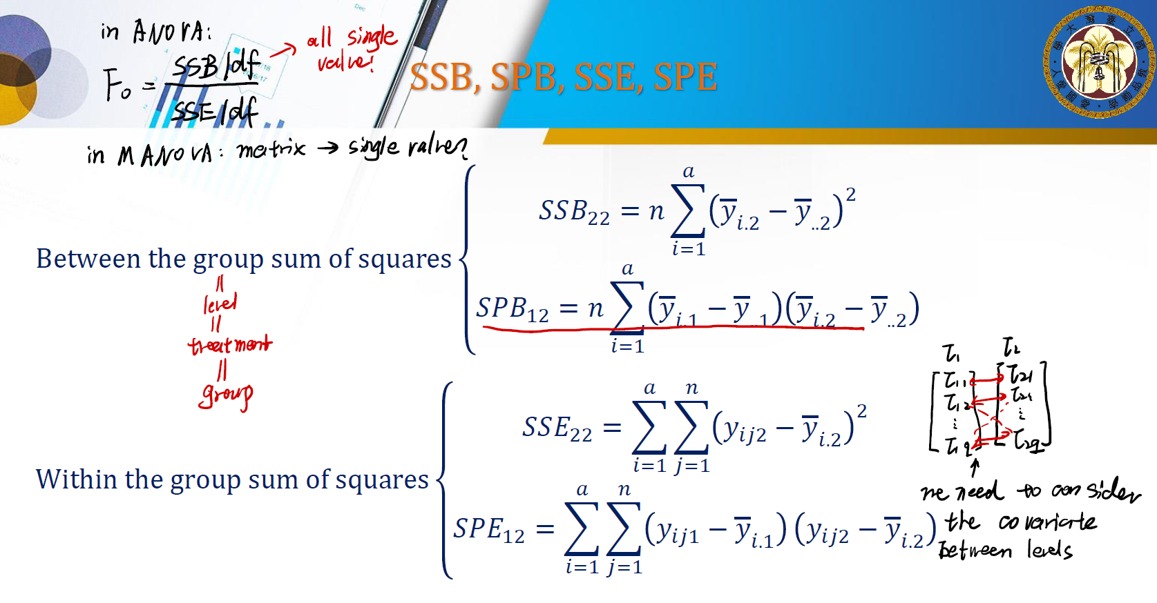
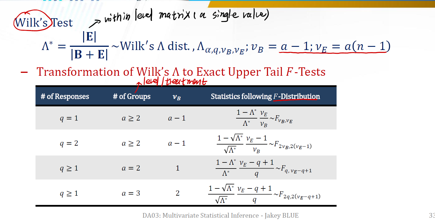
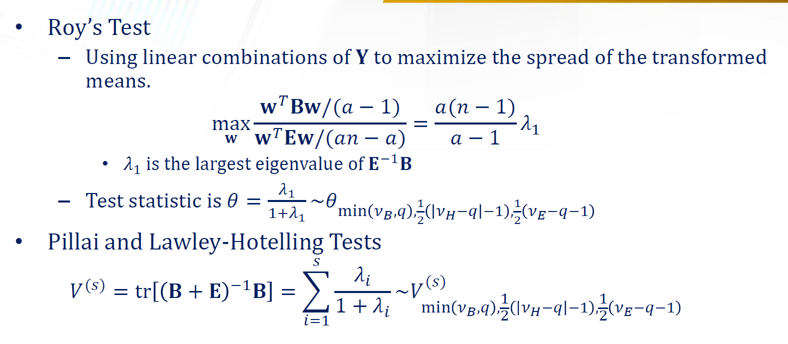
Testing Statistics of MANOVA
在 MANOVA 中,检定统计量也发生了变化,有多种检定统计量可以使用。
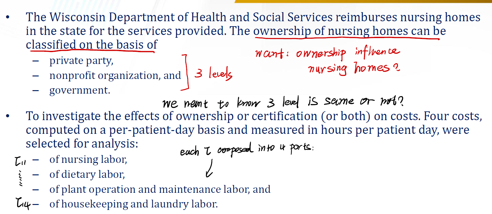
Example: Nursing Home Costs versus Ownership
在这个例子中,我们有3个 level 。其中每个 level 由4个 part 组成。这是一个典型的 MANOVA 分析的问题。
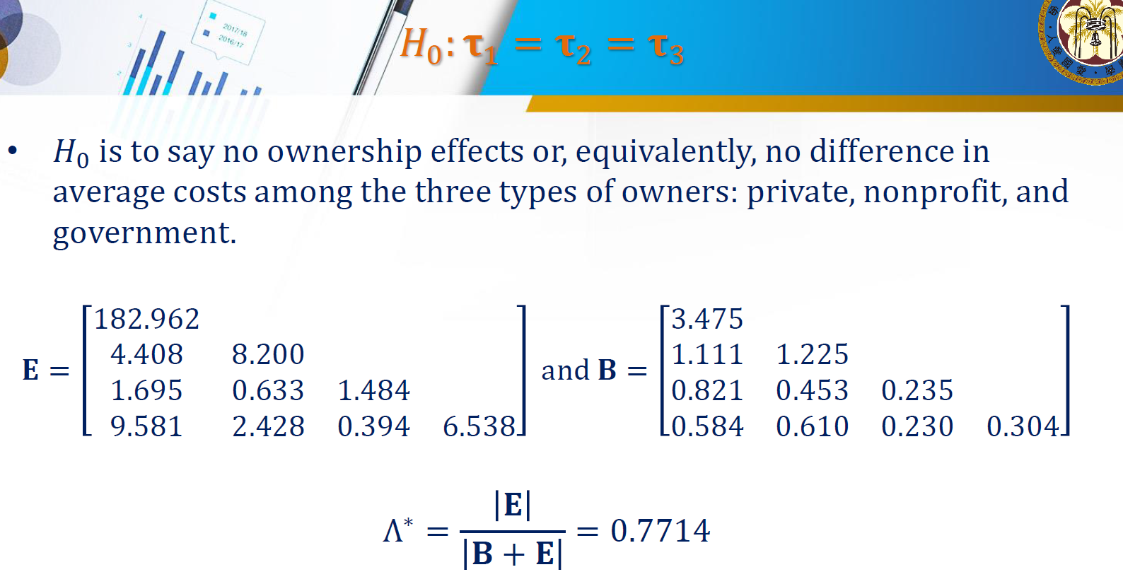
可以直接进行检定:
假设为 $\tau_1 = \tau_2 = \tau_3$
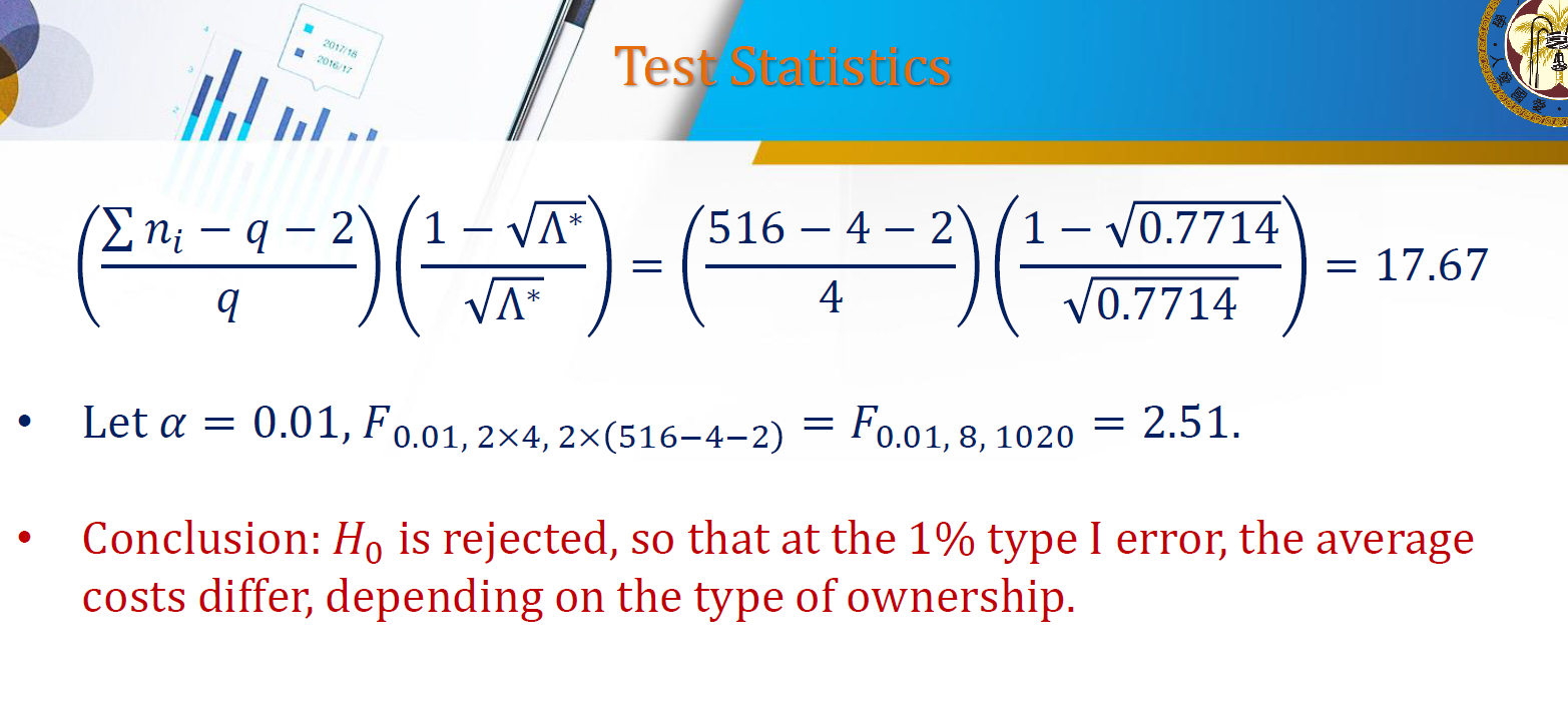
以上,就是 MANOVA 的相关内容。
Reference
本文中的所有图片,Slides均来源于國立台灣大學工業工程學研究所藍俊宏副教授所開設的資料分析方法課程中之 DA03 Multivariate Statistical Inference.pdf。特此感謝藍俊宏老師在我學習歷程上的幫助!